| Commands | Description | |
| ActiveCell.CurrentRegion.Select | Select a range or block of data (Cells). Keep columns to the left and right clear of data so that they are not apart of the block. | |
| Selection.End(xlDown).Select |
End down | |
| ActiveCell.Offset(1, 0).Select | offset (Row, Col) | |
| ActiveSheet.DisplayPageBreaks = False | Removes dotted print lines | |
| Application.DisplayAlerts = False | Turn alert alerts On (=True) or Off (=False) example | |
| Application.ScreenUpdating = False | This is used so that you do not see the macro run.
It makes the macro go faster. Note if you use this the cursor will not follow you to the new cell. |
|
| Application.CutCopyMode = False | This is like pressing “Esc” to get rid of the rubber band box. Use this after you have pasted your data. | |
| ActiveWorkbook.Save ActiveWorkbook.Close Savechanges:=True |
This will save the workbook This will close and save the workbook |
|
| ActiveCell.EntireColumn.AutoFit | Adjust current column width | |
| ActiveCell.EntireColumn.Copy | copy active column | |
| Sheets("Sheet3").Select | Go to sheet 3 | |
| [a1].Select | Go to a Cell location - If using screen updating the cursor will not follow to active cell | |
| Range("A1:D20").Select | Select a Range of cells | |
| Selection.Copy | Copy Active Selection | |
| ActiveSheet.Paste | Paste data to ActiveCell | |
| vbCrLf replace with VBNEWLINE |
This will add a Carrage Return in VBA used to start a new line of data MsgBox = "First Line & vbCrLf & Second Line" |
|
| Turn on and off the caluculation function | Application.Calculation = xlManual Application.Calculation = xlAutomatic |
|
| Minus Minus in front of a formula. =IsNumber( ) ' would result in either True or False =--IsNumber( ) ' would result in either 0 or 1 |
=ISNUMBER(IFERROR(SEARCH($B$3,E3,1),"")) |
|
| How to add a Key Stroke to activate a macro. | Click Developer tab / click on Macros / click Options |
| w3School web site |
Folder Names to Text File
-
To list folder names into a *.txt file, you can use the Command Prompt or PowerShell. Here are the steps for each method:
Using Command Prompt:
Open Command Prompt and navigate to the directory containing the folders you want to list.
Enter the command dir /ad /s /b > folderlist.txt to create a text file named folderlist.txt that includes all folder names, including subfolders.
Using PowerShell:
Open PowerShell and navigate to the directory containing the folders you want to list.
Enter the command Get-ChildItem -Directory -Recurse | Select-Object -ExpandProperty Name > folderlist.txt to create a text file named folderlist.txt that includes all folder names, including subfolders.
Alternatively, you can modify the context menu to add a "Copy Folder List to Clipboard" option, which you can then paste into a text file. To do this, you need to edit the registry and add the command cmd /c dir "%1" /a:-d /o:n | clip to the context menu entry.
For a simpler method, you can also use a batch file with the command dir /ad /s /b > folderlist.txt to automatically generate the folder list in a text file.
BAR Codes using excel
-
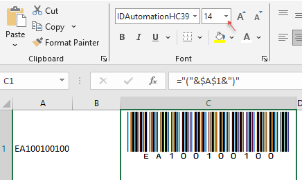
Download IDAutomationHC39M Free Version ... Get it here
UIse the font installer to install the font.
In excel Cell A1. Enter EA100100100 in the Cell. In cell C1 enter: ="("&A1&")"
The barcode should be set for a minimum of 14px
Substitute Split Numbers and Letters in a Serial number
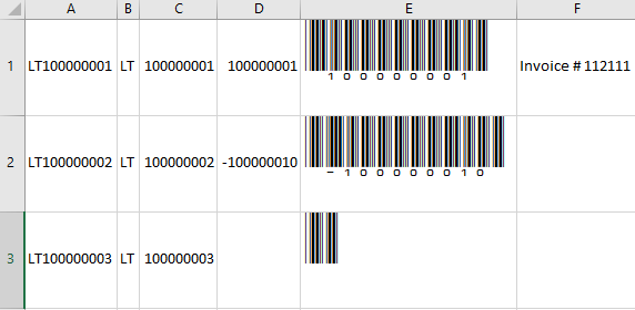
In this example the serial number LT100000001 is located in cell A1
Cell B1 will contain the following formula:
[B1].Formula = "=(SUBSTITUTE(SUBSTITUTE(SUBSTITUTE(SUBSTITUTE(SUBSTITUTE(SUBSTITUTE(SUBSTITUTE(SUBSTITUTE(SUBSTITUTE(SUBSTITUTE(A1,""0"",""""),""1"",),""2"",),""3"",),""4"",),""5"",),""6"",),""7"",),""8"",),""9"",))"
Cell C1 will contain the following formula:
[C1].Formula = "=VALUE(SUBSTITUTE(SUBSTITUTE(SUBSTITUTE(SUBSTITUTE(SUBSTITUTE(SUBSTITUTE(SUBSTITUTE(SUBSTITUTE(SUBSTITUTE(SUBSTITUTE(A1,""A"",""""),""E"",),""Q"",),""P"",),""S"",),""F"",),""J"",),""L"",),""N"",),""T"",))"
Note that the serial number is text so we add VALUE to the Statement. The word SUBSTITUTE is used for each letter to substitute starting in (A1,""A"","""") then all other substitutes ,""E"",)
Find_and_Goto_and_Find_Again
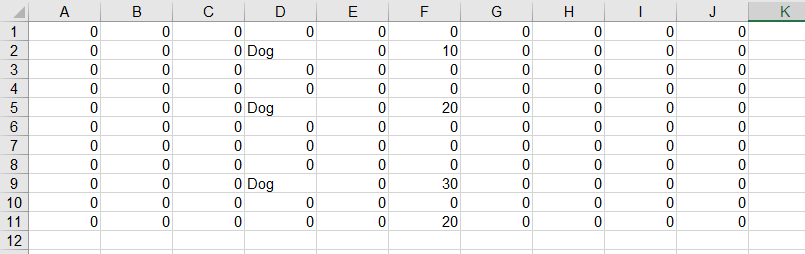
Sub FindNext()
Application.ScreenUpdating = False
Dim rng As Range
Set rng = Range("D:D")
Dim I, U, Y As Variant
U = Application.WorksheetFunction.CountIf(rng, "Dog")
For I = 1 To U
Set rng = Cells.Find(What:="Dog", After:=ActiveCell, LookIn:=xlFormulas, LookAt:= _
xlPart, SearchOrder:=xlByRows, SearchDirection:=xlNext, MatchCase:=False _
, SearchFormat:=False)
If Not rng Is Nothing Then
rng.Select
U = ActiveCell.Row
Y = Cells(U, 6)
' MsgBox Y ' this just confirms the value of the offset and is not needed
'Else
' MsgBox "not found"
End If
Next I
End Sub
Move data from one workbook to another workbook
Sub DB()Dim A, B, C, D, E, F, G, H, i, J, K, L, LP, M, N, O, P, Q, R, S, T, U, V, W, X, Y, Z As String
Dim dt As Date
dt = Date
Dim DB1 As Workbook
Dim DB As Workbook
Set DB = Workbooks.Open("L:\AMC_TestResults\OpticTesting\OpticTestingR8.1.xlsm")
A = Cells(2, 1) 'invoice
B = Cells(1, 3) 'StockID
Dim RNG As Range
Set RNG = Range("B:B")
Z = Application.WorksheetFunction.CountIf(RNG, "Xcvr") + 7
C = Range(Cells(8, 5), Cells(Z, 6)).Copy 'SN and PN
Cells(8, 1).Select
Do Until (ActiveCell = "Physical")
ActiveCell.End(xlDown).Select
Loop
D = ActiveCell.Offset(23, 11)
E = ActiveCell.Offset(24, 11)
F = ActiveCell.Offset(27, 11)
G = ActiveCell.Offset(28, 11)
H = ActiveCell.Offset(37, 8)
i = ActiveCell.Offset(38, 8)
J = ActiveCell.Offset(52, 8)
K = ActiveCell.Offset(53, 8)
L = ActiveCell.Offset(67, 8)
M = ActiveCell.Offset(68, 8)
N = ActiveCell.Offset(82, 8)
O = ActiveCell.Offset(83, 8)
Set DB1 = Workbooks.Open("L:\AMC_TestResults\OpticTesting\TestingDB.xlsm")
DB1.Sheets("Home").Range("A1").End(xlDown).Offset(1) = dt
DB1.Sheets("Home").Range("B1").End(xlDown).Offset(1) = A
DB1.Sheets("Home").Range("C1").End(xlDown).Offset(1) = B
DB1.Sheets("Home").Range("D1").End(xlDown).Offset(1).PasteSpecial
DB1.Sheets("Home").Range("F1").End(xlDown).Offset(1) = D
DB1.Sheets("Home").Range("G1").End(xlDown).Offset(1) = E
DB1.Sheets("Home").Range("H1").End(xlDown).Offset(1) = F
DB1.Sheets("Home").Range("I1").End(xlDown).Offset(1) = G
DB1.Sheets("Home").Range("J1").End(xlDown).Offset(1) = H
DB1.Sheets("Home").Range("K1").End(xlDown).Offset(1) = i
DB1.Sheets("Home").Range("L1").End(xlDown).Offset(1) = J
DB1.Sheets("Home").Range("M1").End(xlDown).Offset(1) = K
DB1.Sheets("Home").Range("N1").End(xlDown).Offset(1) = L
DB1.Sheets("Home").Range("O1").End(xlDown).Offset(1) = M
DB1.Sheets("Home").Range("P1").End(xlDown).Offset(1) = N
DB1.Sheets("Home").Range("Q1").End(xlDown).Offset(1) = O
Cells(2, 4).End(xlDown).Offset(0, -3).Select
If ActiveCell <> "" Then
GoTo line1
End If
Cells(2, 4).End(xlDown).Offset(0, -3).Select
Range(Selection, Selection.End(xlUp)).FillDown
ActiveCell.Offset(0, 1).Select
Range(Selection, Selection.End(xlUp)).FillDown
ActiveCell.Offset(0, 1).Select
Range(Selection, Selection.End(xlUp)).FillDown
ActiveCell.Offset(0, 3).Select
For T = 1 To 12
ActiveCell.End(xlUp).Offset(1) = "."
Range(Selection, Selection.End(xlUp)).FillDown
ActiveCell.Offset(0, 1).Select
Next T
Do Until (ActiveCell = "")
Cells(3, 6).Select
If ActiveCell <> "." Then
ActiveCell.Interior.ColorIndex = 4
ActiveCell.Offset(1).Select
End If
Loop [A1].Select line1: End Sub
Find Next Tx
- Sub FindnextTx()
Dim i, x As Integer
Dim rng, columnRange, cellToFind, foundCell As Range
Set rng = Range("B:B")
x = Application.WorksheetFunction.CountIf(rng, "Tx")
'You can do a (for loop) or a (Do until loop)
For i = 1 To x
'Set the column range to search
Set columnRange = Range("B:B")
'Get the cell value to find
cellToFind = "Tx"
'Find the cell in the column range
Set foundCell = columnRange.Find(what:=cellToFind, LookIn:=xlValues, LookAt:=xlWhole, SearchOrder:=xlByRows, SearchDirection:=xlNext, MatchCase:=False, searchformat:=False)
'If the cell was found, go to that cell address
If Not foundCell Is Nothing Then
foundCell.Activate
End If
'Do other things like putting Rx in the cell 1 column to the right
ActiveCell.Offset(0, 1) = "Rx"
ActiveCell = "Txx"
Next i
End Sub
Find Cell by color
- =LOOKUP(2,1/($A$1:$C$100=I1),$C$1:$C$100)
=LOOKUP(2,1/(Range = Criteria),Range gets the answer from)
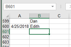
Looking up the last row number where cell E1 = EdithA B C D E 1 Dan 1 Edith 2 Edith 2 3 Dan 3 4 Edith 4 - The solution is hidden on the "Review" tab in the "Changes" ribbon. There is a button called "Allow Users to Edit Ranges". You need to protect the sheet from this window.
-
Dim rng as Range
Set rng = wsS.Range("Table2[#Retail]") - Open the Excel spreadsheet containing the data you want to display in your Word document.
- Select the data you want to appear in the Word document and press "Ctrl-C" to copy it.
- Launch Microsoft Word and open the document in which you wish to display the data.
- Place the cursor in the area of the Word document where you want the Excel data to be displayed and right-click. Choose either "Link & Keep Source Formatting" or "Link & Use Destination Styles" depending on whether you want to use the formatting and style options from the original Excel file or the Word document respectively.
- Save your documents. From now on, when you update the Excel file, the table in Word will also be updated. Be aware, however, that you will need to repeat the previous steps if you change the location or name of the Excel file.
-
Sub export_excel_to_word()
Dim objWord As New Word.Application
'Copy the range Which you want to paste in a New Word Document
Range("A1:B10").Copy
With objWord
.Documents.Add "Y:\Edith\OCSkinINTHEBUFF_Receipt.docx"
.Selection.Paste
.Visible = True
End With
End Sub
- Worksheets("Records").DropDowns("Drop Down 1") = 1
- ComboBox1.ListIndex = 0
or change the target cell to 0 ... [A1] = 0 - Click here
-
Sub scrll()
Dim x As Integer
x = [A1]
ActiveWindow.ScrollRow = x
ActiveWindow.ScrollColumn = x
End Sub - This is controlled using the "SelectionChange" Event on the sheet not in a module.
- There is an "OFF" and "ON" so that players names can be chanaged. Off & On turn off and on the event handler.
- Winner is aConditional Format
-
Sub Uppercase()
Dim rng As Range
Dim cell As Variant
'Set rng = selection (Use this line to select a range)
Set rng = Range("K17:K26") 'Use this line for a static range
For Each cell In rng
cell.Value = UCase(cell)
Next
End Sub
Sub lowercase()
Dim rng As Range
Dim cell As Variant
'Set rng = selection (Use this line to select a range)
Set rng = Range("K17:K26") 'Use this line for a static range
For Each cell In rng
cell.Value = lcase(cell)
Next
End Sub
Sub ProperCase()
Dim rng As Range
Dim cell As Variant
'Set rng = selection (Use this line to select a range)
Set rng = Range("K17:K26") 'Use this line for a static range
For Each cell In rng
cell.Value = Application.WorksheetFunction.Proper(cell)
Next
End Sub
-
Sub hide()
Sheet3.Visible = False
Sheet4.Visible = False
Sheet5.Visible = False
' You can hide as many sheets as you like.
End Sub
Sub Unhide()
Sheet3.Visible = True
Sheet4.Visible = True
Sheet5.Visible = True
End Sub
- Copy the data from sheet 1 to sheet2 and transpose the data into columns
- Set a & b range for column "A"
- Goto an open cell and concatenate using "ActiveCell = a & b". Once the loop is complete Delete column "A" to shift all data to the left and start loop "P"
- Once loop "P" is complete macro will copy all data and paste to sheet 3 using transpose to put data back into rows.
- Introduction
- Sheets and Cells
- Variables
- Conditions
- Loops
- Proceedures and Function
- Dialog boxes
- Events
- Forms and controls
- Arrays
- Supplements
- Create a worksheet named “Menu” that serves as a menu page. On that page, add a button that will control the macro.
- Create the macro, here is the Code.
Sub openws()
Dim xinput As Variant
Dim ws As Worksheet
xinput = InputBox("Enter your password")
Select Case xinput
Case "pw2" 'This is the password for this sheet
Sheets("Sheet2").Visible = True
Sheets("Sheet2").Activate
Case "pw3"
Sheets("Sheet3").Visible = True
Sheets("Sheet3").Activate
Case "pw4"
Sheets("Sheet4").Visible = True
Sheets("Sheet4").Activate
Case "Showall" 'this should be a Very Strong Password
For Each ws In ActiveWorkbook.Worksheets
ws.Visible = True
Next
Case "Hideall" 'this will hide all worksheets
For Each ws In ActiveWorkbook.Worksheets
If ws.Name <> "Menu" Then
ws.Visible = xlVeryHidden
End If
Next
Case Else
MsgBox "Incorrect Password", vbExclamation
End Select
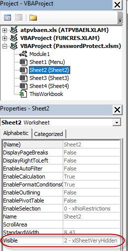
End Sub - For each worksheet change (-1xlSheetVisable) to (2-xlSheetVeryHidden)
in the VBA editor. - Place the activecell in column "A".
- Press "F5"
- Choose Special
- Click "Blanks"
- Click "OK"
- In formula bar type: =B2
- Press: Ctrl + Enter
- =sum(Todays Date - Birthday)/365.25
- You Tube Link
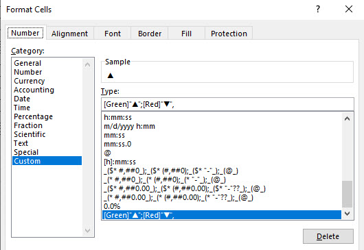
Basic custom formating- How Positive numbers should be formated ;
- How Negitive numbers should be formated ;
- How Zero's should be formated ;
- How Text should be formated ;
- # Hash tag is a numerical placeholder
- ; - SemiColin is as a separator
- Up/Down Arrows. Get from "Inset tab" Symbols and place them in a cell somewhere. To use these synbols you must vopy them from the "Formula bar" and noto the cell you placed them in.
- Adding color to the symbol
use square brackets [Color10] like this or to add any color from the Microsoft color pallet.
Find Cell by color
-
This will go to each cell and check the color, if it is equal to 65535 (Yellow)
it will print the value in the immediate window. You could amend the code to put
the values elsewhere. Hope this helps.
Range("O3").Select
Do While ActiveCell.Value <> ""
If ActiveCell.Interior.Color = 65535 Then
Debug.Print ActiveCell.Value
End If
ActiveCell.Offset(1, 0).Select
Loop
Change a range of cells Case to Upper, Lower or Proper
-
Dim R as Integer
Dim rng1 as Range, rng2 As Range, cell as Range
Set rng1 = Range("A:A")
R = Application.WorksheetFunction.CountA(rng1)
Set rng2 = Range("A1:A" & R)
For Each cell In rng2
cell.value = WorksheetFunction.Proper(cell.value)
Next cell
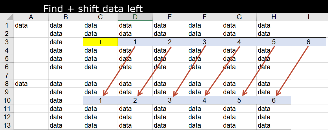
Find "+" in column "C" and shift data to the left
- Sub LocateAndGoToCell()
'Declare variables
Dim AR, cnt, i As Integer
Dim rng As Range
Dim columnRange As Range
Dim cellToFind As String
Dim foundCell As Range
Set rng = Range("A:A")
cnt = Application.WorksheetFunction.CountA(rng)
'Set the column range to search
Set columnRange = Range("C:C")
'Get the cell value to find
cellToFind = "+"
'Find the cell in the column range
For i = 1 To cnt
Set foundCell = columnRange.Find(What:=cellToFind, LookIn:=xlValues, LookAt:=xlWhole, SearchOrder:=xlByRows, SearchDirection:=xlNext, MatchCase:=False, SearchFormat:=False)
'If the cell was found, go to that cell address
If Not foundCell Is Nothing Then
foundCell.Activate
AR = ActiveCell.Row
Range(Cells(AR, 4), Cells(AR, 10)).Cut Cells(AR, 3)
End If
Next i
End Sub
This example uses the Left function to return a specified number of characters from the left side of a string.
- Dim AnyString, MyStr
AnyString = "Hello World" ' Define string.
MyStr = Left(AnyString, 1) ' Returns "H".
MyStr = Left(AnyString, 7) ' Returns "Hello W".
MyStr = Left(AnyString, 20) ' Returns "Hello World".
Open Windows Explorer to specific folder
-
Sub results()
Dim spath As String
spath = "L:\AMC_TestResults"
Shell "C:\WINDOWS\explorer.exe """ & spath & "", vbNormalFocus
End Sub
Keyboard shortcuts
Link to Frequently used shortcuts
-
Example:
ALT + = will sum a row or column
Uppercase a range with VBA
- ' Upper CASE
Dim rng As Range
Set rng = Range("A1:E10000")
rng = Evaluate("index(upper(" & rng.Address & "),)")
Print Page to PDF
- Dim path As String
path = "E:\Crystalpdf"
wsCOC.Activate
wsCOC.Range("A1:D31").Select
ActiveSheet.ExportAsFixedFormat Type:=xlTypePDF, Filename:= _
path & "/" & Inv & ".pdf", Quality:=xlQualityStandard, _
IncludeDocProperties:=True, IgnorePrintAreas:=False, OpenAfterPublish:= _True
'Need to Save TO pdf (Example 2)
Dim path As String
path = "L:\PickBarCodes"
wsB.Range("A1").CurrentRegion.Select
ActiveSheet.ExportAsFixedFormat Type:=xlTypePDF, filename:=path & "/" & inv & ".pdf", Quality:=xlQualityStandard, _
IncludeDocProperties:=True, IgnorePrintAreas:=False, OpenAfterPublish:=True
Convert text to number
Find a cell by its color
- Sub FindLastColoredCell()
'PURPOSE: Determine Last Cell On Sheet Containing Specific Fill Color
'AUTHOR: Rick Rothstein
'SOURCE: www.TheSpreadsheetGuru.com/the-code-vault
'Ensure Find Formatting Rule is Reset
Application.FindFormat.Clear
'Store active cell's fill color into "Find"
Application.FindFormat.Interior.Color = ActiveCell.Interior.Color
'Notify User of location using the "Find" Action
MsgBox "Last Color Found: " & ActiveSheet.UsedRange.Find("", , , , , xlPrevious, , , True).Address
'Reset Find Formatting Rule
Application.FindFormat.Clear
End Sub
Message Box Timer
-
Sub TimedMessage As String = "Testing Optic Components Completed()
Const Title"
Const Delay As Byte = 2 ' show timeout in seconds
Const wButtons As Integer = 16 ' buttons and Icons
Dim wsh As Object, msg As String
Set wsh = CreateObject("WScript.Shell")
msg = Space(10) & "All Parts Tested Successfully"
wsh.Popup msg, Delay, Title, wButtons
Set wsh = Nothing
End Sub
Match for Row Number from the bottom up
Protected Sheet will not protect
Setting up a dynamic range using a table
How To Automate a Table in Word Using Excel
-
This saves manually updating the contents of both an Excel spreadsheet and a Word document separately. After you have completed the following steps, the table in Word will be automatically updated whenever you change the data in the Excel spreadsheet document.
Copy from Excel to Word
Reset Dropdown lists
Reset Combo Box
Password Protect a Button
-
Add this to the top of your macro
Dim MyPassword As String
MyPassword = "zebra"
If InputBox("Please enter password to continue.", "Enter Password") <> MyPassword Then
MsgBox ("Wrong Password. Try Again")
Exit Sub
End if
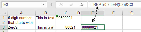
=REPT(0,8-len(A1))&A1 ...Put Zero's 0 in front of numbers.
While loop
-
'-Places Data in Finish Cells Column B --------------------
[E1].Select
Do
While Cells(x, 2) = ""
tiveCell.Offset(1).Select
If ActiveCell = t Then
Cells(x, 2) = ActiveCell.Offset(-1, 1)
x = x + 4
t = t + 1
End If
If ActiveCell = "" Then Cells(x, 2) = ActiveCell.Offset(-1, 1)
If ActiveCell = "" Then Exit Do
Wend
x = x + 1
Loop
-
Here is more information on loops
Another example:
'St = Starting Row number
- Do Until ActiveCell = "SN"
ActiveCell.Offset(-1).Select
Loop
ActiveCell.Offset(1).Select
St = ActiveCell.Row
'Ed = Ending Row number
Do Until ActiveCell = "JDAN"
ActiveCell.Offset(1).Select
Loop
ActiveCell.Offset(-1).Select
Ed = ActiveCell.Row
Send email from excel
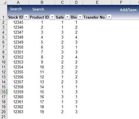
StockID Searchable Table
Scroll
Copy and paste End(xldown)
-
Dim r As Long
Dim rng As Range
Set rng = Range("D:D")
r = Application.WorksheetFunction.CountA(rng)
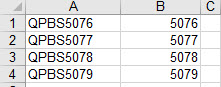
'Write formula for E
Cells(1, 5).Formula = "=right(D1,4)"
Range("E1").Select
Selection.AutoFill Destination:=Range("E1:E" & r)
Copy and Paste a range
Sub copy1()
'This copies To "A" From "C"
Dim LRow As Integer
Dim RNG As Range
Set RNG = Range("C1:C50000")
LRow = Application.WorksheetFunction.CountA(RNG)
Range("A1:A" & LRow).Value = Range("C1:C" & LRow).Value
End Sub
Sub copy2()
'This copies To "A" From "C"
Dim LRow As Integer
Dim RNG As Range
Set RNG = Range("C1:C50000")
LRow = Application.WorksheetFunction.CountA(RNG)
Range("G1:I" & LRow).Value = Range("A1:C" & LRow).Value
End Sub
How to stop a running macro
-
Press ESC repeatedly
Press Ctrl Break
or
It may happen that, both Escape or Ctrl+Break button may not work for you. As your Macro may have “Application.EnableCancelKey = xlDisabled”
command line which may not allow you to interrupt the ongoing Macro command. In such a case, you can simply remove this line of an item and add a new command line – “Application.EnableCancelKey = xlInterrupt”
It will allow you to interrupt the ongoing Macro command
BarCodes for Excel
-
Download and install
Cell A1 contains the data for the barcode
Cell B1 will contain the formula: ="("A1&")"
Cell B1 select, and change font to "IdAutomationHC39M Free Ver"
After Enter Move to cell (Up, Down, Left, Right
'*****CODE FOR SHEET1*****Option Explicit
Private Sub Worksheet_Activate()
- Application.MoveAfterReturnDirection = xlToRight
Application.MoveAfterReturnDirection = xlToLeft
Application.MoveAfterReturnDirection = xlUp
Application.MoveAfterReturnDirection = xlDown
End Sub
'*************************
Append & Remove data based on cell A1
A |
B |
C |
|
1 |
PartNumber-8pack | Remove -8pack | Append -8pack to B2 |
2 |
Formula | =Left(A1,FIND("-",A1)-1) | =B2&"-8pack" |
3 |
Result | PartNumber | PartNumber-8pack |
Confirm the active cell is in column "A:A"
-
Sub NotInColA()
- If Intersect(ActiveCell, Columns("A:A")) Is Nothing Then
[A1].End(xlDown).Offset(1).Select
End If
Intersect in a specific Range
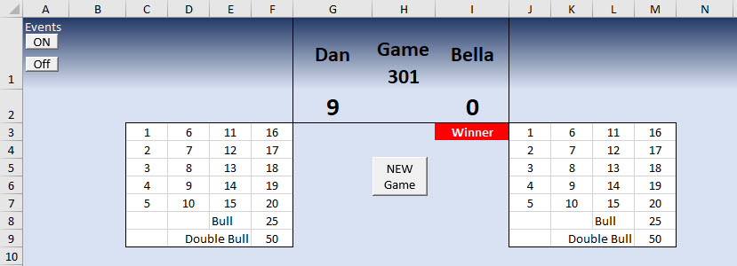
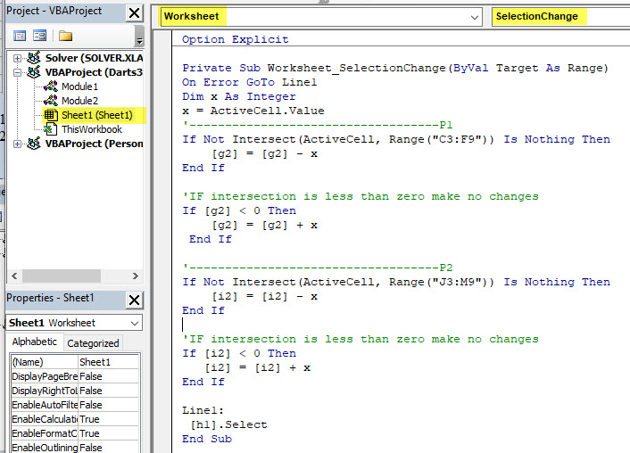
Private Sub Worksheet_SelectionChange(ByVal Target As Range)
On Error GoTo Line1
Dim x As Integer
x = ActiveCell.Value
'-----------------------------------P1
If Not Intersect(ActiveCell, Range("C3:F9")) Is Nothing Then
[g2] = [g2] - x
End If
If [g2] < 0 Then
[g2] = [g2] + x
End If
'-----------------------------------P2
If Not Intersect(ActiveCell, Range("J3:M9")) Is Nothing Then
[i2] = [i2] - x
End If
If [i2] < 0 Then
[i2] = [i2] + x
End If
Line1:
[h1].Select
End Sub
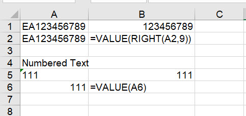
Convert existing text that looks like a number to a number
- Sub ConvertString2Numbers
Dim myVar As Variant
myVar = [B1] ' or Cells(R,C)
Dim FinalNumber as integer
- if Isnumber(myVar) then
finalNumber = CInt(myVar)
Else
finalnumber = 0
End if
[C1] = finalNumber 'This will place the String in cell B1 to C1 as a number.
Convert the String "ABCD1234" in Cell A1 to only the numbers "1234" in B1
- Dim cntA, rw, i, x As Integer
Dim rng As Range
Set rng = Range("A:A")
cntA = Application.WorksheetFunction.CountA(rng)
rw = 1
x = InputBox("Enter Number of numbers")
' This writes the formula =Right(A1,x) where x is a input variable
' Also note that the output is a number and not a String like in the example above.
For i = 1 To cntA
- Cells(rw, 2) = Right(Cells(rw, 1), x)
rw = rw + 1
'Note this will copy down from B1 to CountA of column "A"
VLookup in VBA
- Need to use a helper cell K1 in this case.
- Dim rng As Range
Set rng = Range("A:B")
x = Application.WorksheetFunction.VLookup([k1], rng, 0, False)
Sub VLOO()
Dim X As String
Dim Z As Integer
Dim rng As Range
Set rng = Range("A:B")
Z = InputBox("Enter a number to lookup")
X = Application.WorksheetFunction.VLookup(Z, rng, 2, False)
MsgBox X
End Sub
Using Match to find the row number of an item
- Notice you will need to use a helper cell [Z1].
- r = Application.WorksheetFunction.Match([Z1], rng, 0)
Change UPPPERCASE / lower case / ProperCase
Force Upper Lower and Proper case when using a Inputbox.
-
Sub Uppercase()
Dim a, b As String
a = InputBox("Enter Your name")
b = UCase(a)
MsgBox b
End Sub
Sub Proper()
Dim a, b As String
a = InputBox("Enter Your name")
b = Application.WorksheetFunction.Proper(a)
MsgBox b
End Sub
Sub Lowercase()
Dim a, b As String
a = InputBox("Enter Your name")
b = LCase(a)
MsgBox b
End Sub>
Delete the active row using vba
- Rows(ActiveCell.Row).EntireRow.Delete
Place a formula in a cell
- [A1].Formula = "=Hex2Dec((A3))"
Sub EntrFormulaInCellC1()
'In this example the Formula is entered in Cell C1
Cells(1, 3).ClearContents
[C1].Formula = "=sum(A1+B1)"
End Sub
Sub EntrResultInCellC1()
'In this example the Result is entered in Cell C1
Cells(1, 3).ClearContents
Dim a, b, c As Integer
a = Cells(1, 1)
b = Cells(1, 2)
c = a + b
Cells(1, 3) = c
End Sub
Copy a folders content to another folder
- (Source: http://vba-tutorial.com/copy-a-folder-and-all-of-its-contents/)
Sub chnge1()
Dim path0, path1, path2, Path3 As String
Dim Oldd As Variant
Dim neww As Variant
Dim cnt, i, r As Integer
Dim rng As Range
Set rng = Range("A:A")
r = 1
cnt = Application.WorksheetFunction.CountA(rng)
Oldd = Cells(r, 1)
neww = Cells(r, 2) & ".png"
path0 = "E:\AA_Change\Humm"
path1 = "E:\AA_Change\Dude"
' Copy Humm to Dude
Dim objFSO As Object
Set objFSO = CreateObject("Scripting.FileSystemObject")
objFSO.copyFolder path0, path1
' Change file names from old to new
For i = 1 To cnt
path2 = "E:\AA_Change\Dude" & "\" & Oldd
Path3 = "E:\AA_Change\Dude" & "\" & neww
Name path2 As Path3
r = r + 1
Oldd = Cells(r, 1)
neww = Cells(r, 2) & ".png"
Next i
End Sub
Advanced Filters in a macro 1
Sub autoStockID()
' This will search and sort by Stock ID
On Error GoTo Line1
Dim x As Double
Dim rng As Range
Set rng = Range("A:E")
x = InputBox("Enter Product ID 5 Digit Number")
rng.autofilter Field:=2 ' This clears Field 2
rng.autofilter Field:=1, Criteria1:=x ' This filters the field to "x"
Columns(rng).AutoFit
Line1:
End Sub
Advanced Filters in a macro 2
-
Sub advancedTablefilter()
- Range("K1:N50").Clear
Range("Table1[#All]").Select
Range("Table1[#All]").AdvancedFilter Action:=xlFilterCopy, CriteriaRange:= _
Range("F1:I2"), CopyToRange:=Range("K1"), Unique:=False
Range("F2:I2").Clear
Range("J1").Select
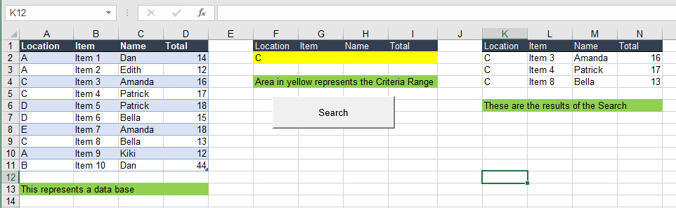
Rather than copying this code to your new macro I would record the macro and then clean it up.
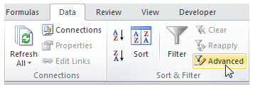 |
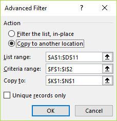 |
| On the "Data tab" you will find Advanced button. | For this set up use "Copy to another location". |
While recording the macro you can have the database on sheet1 and the Criteria on another sheet however the results must reside on the same sheet as the database.
A work around would be to hide the database columns "A:D"
Halt an Event.
The event macro below (UnProtect and Re-Protect) needed to be temporary halted to run another macro. We can temporary halt the event like this
- Application.EnableEvents = False ' This turns the events off
Application.EnableEvents = True
Temporary Unprotect and Re-Protect the Sheet
-
In this macro we halted the running of the Private sub to autofit the rows. Then we turn back on the event.
Private Sub Worksheet_SelectionChange(ByVal Target As Range)
Application.ScreenUpdating = False
ActiveCell.Copy
Worksheets("List").Range("G8").PasteSpecial Paste:=xlPasteValues
ActiveSheet.Unprotect ' Here we unprotect the sheet
Rows("3:51").EntireRow.AutoFit
ActiveSheet.protect DrawingObjects:=True, Contents:=True, Scenarios:=True . 'Here were re-protect the sheet
Application.CutCopyMode = False
End Sub
Hide Columns with a macro XFD is the last column in Excel 2106
-
Sub HidColumns()
- Columns("D:XFD").EntireColumn.Hidden = False
'Columns("D:XFD").EntireColumn.Hidden = True
Columns("A:I").EntireColumn.Hidden = False
'Columns("A:I").EntireColumn.Hidden = True
Hide rows with a macro
- Sub HidRowsYes()
Dim lrow, x As Long
Dim rng As Range
lrow = Cells(Rows.Count, "A").Row
Set r = Range("A1:A" & lrow)
x = Application.WorksheetFunction.CountA(rng) + 1
' Range(Cells(x, 1), Cells(lrow, 1)).Rows.EntireRow.Hidden = True
UnHide rows with a macro
- Sub HidRowsNo()
- Dim lrow, x As Long
Dim r As Range
Set r = Range("A1:A1048576")
lrow = Cells(Rows.Count, "AA").Row
x = Application.WorksheetFunction.CountA(r) + 1
Range(Cells(x, 1), Cells(lrow, 1)).Rows.EntireRow.Hidden = False
' Range(Cells(x, 1), Cells(lrow, 1)).Rows.EntireRow.Hidden = True
Hide / Unhide Sheets
Highlighting a range that meet specific criteria using vba from activecell to an other cell
-
In this example will will skip all cells with 0 zero. and fill cells interior color in range using Select Case as qualifier.
Sub rowsautofit()
Dim r, c As Integer
Dim x As String
r = 3
c = 31 ' change this to what ever the starting column number is
Range("S3:U51").Select ' This will clear the range of interior colors before resetting them.
With Selection.Interior
- .Pattern = xlNone
.TintAndShade = 0
.PatternTintAndShade = 0
Cells(r, c).Select
x = ActiveCell
Do Until IsEmpty(ActiveCell)
If x = "0" Then
- ActiveCell.Offset(1).Select
x = ActiveCell
Else
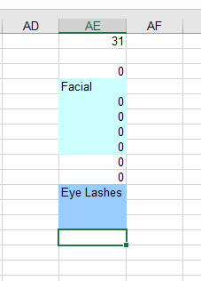
Select Case x ' I am using Case instead of if statements
Case "Facial" ' This says if the case = "Facial" the select activecell and 4 rows same column will be highlighted color 20
Range(ActiveCell, ActiveCell.Offset(4)).Interior.ColorIndex = 20
ActiveCell.Offset(5).Select ' this will then offset by 5 and the macro will continue to search until the activecell is empty.
x = ActiveCell
Case "Eye Lashes"
Range(ActiveCell, ActiveCell.Offset(2)).Interior.ColorIndex = 37 ' This line is will select the activecell thru the activecell.offset(R1,C1)
ActiveCell.Offset(3).Select
x = ActiveCel
End Select
End If
Loop
End Sub
This macro finds the word "Facial" and "Eye Lashes" and then fill color based on criteria.
Deleting sheets with VBA
-
Sub DeletingA_NamedSheet ()
- Application.DisplayAlerts = False
Worksheets("Sheet1").Delete
Application.DisplayAlerts = True
Delete the last sheet
- Sub DeleteLastSheet()
- Application.DisplayAlerts = False
Sheets(Sheets.Count).Delete
Application.DisplayAlerts = True
Copy and paste
Intelli Scense
-
Use ( Ctrl + Spacebar ) to open intelli scense at any time
Hi-Lite 4 rows - (Click here for video)
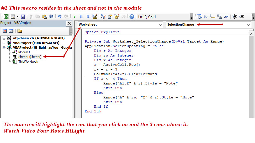
- Sub hilite4rows()
Application.ScreenUpdating = False
Dim r As Integer
Dim rw As Integer
Dim x As Integer
r = ActiveCell.Row()
rw = r - 3
Columns("A:Z").ClearFormats
If r <= 4 Then
Range("A1:Z" & r).Style = "Note"
Exit Sub
Else
Range("A" & rw, "Z" & r).Style = "Note"
Exit Sub
End If
End Sub
Filter by Font Size
Sub filtrbysize()
Dim n As Integer
Dim x As Integer
Dim i As Integer
[A1].Select
n = Application.WorksheetFunction.CountA(Columns(1)) 'n is a column
'n = Application.WorksheetFunction.CountA(Range("A1:A100")) ' n is a range
x = ActiveCell.Font.Size
For i = 1 To n
ActiveCell.Offset(0, 1).Value = x
ActiveCell.Offset(1).Select
x = ActiveCell.Font.Size
Next i
Columns("A:B").Select
ActiveWorkbook.Worksheets("Sheet1").Sort.SortFields.Clear
ActiveWorkbook.Worksheets("Sheet1").Sort.SortFields.Add2 Key:=Range("B1:B" & n) _
, SortOn:=xlSortOnValues, Order:=xlDescending, DataOption:=xlSortNormal
With ActiveWorkbook.Worksheets("Sheet1").Sort
.SetRange Range("A1:B" & n)
.Header = xlGuess
.MatchCase = False
.Orientation = xlTopToBottom
.SortMethod = xlPinYin
.Apply
End With
Columns("B:B").ClearContents
[A1].Select
End Sub
UBound Function (Click here for two-dimensional array)
- Return the highest subscript of a one-dimensional array.
Dim prices(0 to 10) As Double
Dim pricesUB As Integer
pricesUB = UBound( prices )
' Now the integer pricesUB has the value 10.
Move to next Tab and call a macro. (These 2 macros work together)
-
Sub nextst()
Dim x As Integer
Dim book As Integer
x = Application.Worksheets.Count - 1 ' This line counts the number of tabs in the workbook less one for the original page
For book = 1 To x
- Worksheets(ActiveSheet.Index + 1).Select ' This moves to the next tab
Call threepercent ' This calls the macro below for the new tab
Worksheets("Summary").Select
ActiveWorkbook.Save
MsgBox "Done!"
End Sub
Sub threepercent()
Dim tms As Integer
Dim r As Integer
Dim c As Integer
Dim i As Integer
Dim prcnt As Double
tms = 17
r = 8
c = 2
Application.ScreenUpdating = False
Range("B8:B25").Copy Destination:=Range("AA8") ' Copies current data to new location
Range("B8:B25").ClearContents
[AA8].Select
prcnt = Application.WorksheetFunction.Sum(ActiveCell * 0.03) + ActiveCell ' Adds 3 percent and copies back to original location
Cells(r, c).Value = prcnt
For i = 1 To tms
- ActiveCell.Offset(1).Select
r = r + 1
prcnt = Application.WorksheetFunction.Sum(ActiveCell * 0.03) + ActiveCell
Cells(r, c).Value = prcnt
Range("AA8:AA25").Clear
[A7].Select
End Sub
Worksheets and Sheets
- Worksheet("Sheet1").select
- This selects the exact sheet named "Sheet1"
Worksheet(2).select
- This would error as there is no "Sheet2"
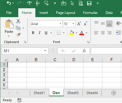
Sheets(2).select
- This refers to the second sheet from the left regardless of the sheet name. In this case Sheet(2) = Dan
Using a simple Math function without using a Function Statement
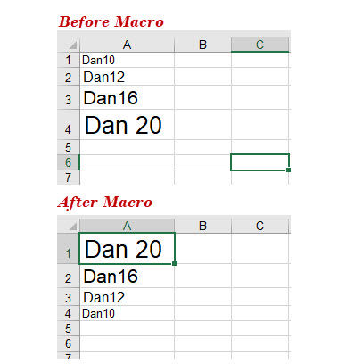
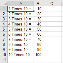
Dim Startnumber As Integer Dim Endnumber As Integer Dim answer As Long Dim Timestable As Integer Endnumber = 10 Timestable = 10 For Startnumber = 1 To Endnumber answer = Startnumber * Endnumber ' Note answer is a math function Cells(Startnumber, 1).Value = Startnumber & " Times " & Timestable & " = " Cells(Startnumber, 1).Offset(, 1).Value = answer Next Startnumber End Sub |
 |
Scroll the Activecell to the "A1" Position
- Dim r As Long
r = ActiveCell.Row()
ActiveWindow.ScrollRow = r
or
ActiveWindow.ScrollColumn = r
Convert Date to Text and Concatenate
-
Sub convert2Text_AND_Concatenate()
- Dim str1 As String
Dim a As String
Dim d As Date
d = Date
a = "Dan"
str1 = Str(d) ' Using "Str", the date is now a string. Note it may need =trim
[c7] = str1 ' C7 now displays the date as Text
' [c7] = "Today's Date is:" & str1 (Note - this can concantenate because both the text and the date are Text)
Concatenate cells W/ VBA
- Sub concat()
Dim a As Variant, b As Variant, c As Variant, x As Variant
a = [a1]
b = [b1]
c = [c1]
x = a & b & c
[E1].Value = x
End Sub
=EoMonth
- Sub ConcatMonthYear2()
- Dim t As Date
Dim x As Date
t = Date
x = WorksheetFunction.EoMonth(t, 1)
[A1] = x
[A1].NumberFormat = "mmm yyyy"
End Sub
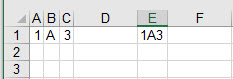
Center Text with out using [Merge&Center]
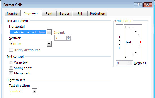 |
Sub CenterAcrossColumns() With Selection
.MergeCells = False End Sub This acts like Merge and Center but does not merge the cells. 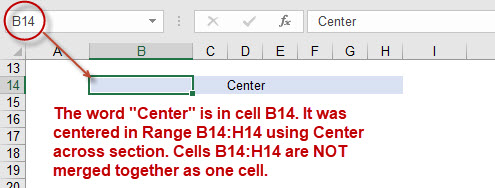 |
Working with Worksheet Functions ...... List of Functions that can be used in Macro's
More info on Macro Functions
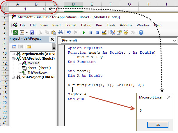
Function and Sub - - - Adding Cells "A1" + "B1"
In this function we are determining if the activecell contains a Number or Not a Number, thus (a Letter) using a Function
| Function CheckCell(CellValue) As Boolean If IsNumeric(CellValue) Then CheckCell = True Else CheckCell = False End If End Function Sub izNumber() Dim ReturnValue As Boolean ReturnValue = CheckCell(ActiveCell.Value) If ReturnValue = False Then MsgBox ("Activecell is Not a number - Exit sub") Else MsgBox "The Activecell is a Number" End If End Sub |
Sub iznumber() End Sub Note that the macro above will not work like the Function and Sub to the left. If we change "Variant" to "Long" the macro will fail if the ActiveCell is a Letter. So, the Function tells us what the ActiveCell is. Is it a Number or is it a Letter and the macro takes the appropriate action? |
WorksheetFunctions Examples
Sub FunctionExample()
Dim n As Long
Dim x As Long
Dim a As Long
Dim b As Long
Dim c As Long
Dim D As Long
Dim E As Long
Dim F As Long
Dim G As Long
Dim diff as long
n = WorksheetFunction.Average(Range("D:D")) 'This section sums columns
x = WorksheetFunction.Sum(Range("D:D"))
a = WorksheetFunction.Sum(Range("D:D")) + 1
b = WorksheetFunction.Sum(Range("D:D")) - 1
c = WorksheetFunction.Sum(Range("D:D")) / 2
D = WorksheetFunction.CountA(Range("D:D"))
E = WorksheetFunction.Min(Range("D:D"))
F = WorksheetFunction.Max(Range("D:D"))
G = WorksheetFunction.Large(Range("D:D"), 2)
diff = Range("B1") - Range("A1") 'diff is like saying =sum(B1-A1) - use this to sum or minus + or / two cells
[i1].Value = x
[i2].Value = n
[i3].Value = a
[i4].Value = b
[i5].Value = D
[i6].Value = E
[i7].Value = F
[i8].Value = G
[i9].value = diff
End Sub
Shift a Column to the right
Sub insertCC()
Dim diff, iCntr As Integer
diff = Range("B1") - Range("A1") + 1
If Cells(1, 1) = "" Or Cells(1, 2) = "" Then ' Here we are using the "OR" command so if (Cell A1 or B1) is empty then
- MsgBox "Missing Data in Cell A1 or B1. Please try again."
Exit Sub
For iCntr = 1 To diff
- Columns("C:C").Insert Shift:=xlToRight ' Note here we can Insert and Shift Column C moving data to the right
Range("C1") = Range("B1") - iCntr + 1
End Sub
Concatenating a Range of cells
-
Answer from web.
       Private Sub Trial_1_Click()

     Dim lr As Long


     lr = Cells(Rows.Count, ActiveCell.Column).End(xlUp).Row

     Select Case lr - ActiveCell.Row

       Case 0: Range("P2").Value = ActiveCell.Value

       Case Is < 0: Range("P2").ClearContents

       Case Else: Range("P2").Value = Join(Application.Transpose(Range(ActiveCell, Cells(lr, ActiveCell.Column))), "")

     End Select

   End Sub
=Concatenate A1,B1 - - A1,C1 -- A1,D1
   Sub Concat1()

   Dim ws1 As Worksheet

   Set ws1 = Worksheets("Sheet1")

   Dim ws2 As Worksheet

   Set ws2 = Worksheets("Sheet2")

   Dim ws3 As Worksheet

   Set ws3 = Worksheets("Sheet3")

   Dim a As Range

   Dim b As Range

   Dim x As Integer

   Dim y As Integer

   Dim i As Long

   Dim lrow As Long

   Dim p As Long

   ws1.Range("A1").CurrentRegion.Copy

   ws2.Range("A1").PasteSpecial Paste:=xlPasteValues, Operation:=xlNone, SkipBlanks:=False, Transpose:=True


   ws2.Select


   For p = 1 To 647

   lrow = Cells(Rows.Count, "A").End(xlUp).Row - 1

   x = 1

   y = 2

   Set a = Range("A" & x)

   Set b = Range("A" & y)

   [XX1].Select

   For i = 1 To lrow


   ActiveCell = a & b

   ActiveCell.Offset(1).Select

   y = y + 1

   Set b = Range("A" & y)

   Next i


   Columns("A").Delete

   Next p


   ws2.Range("A1").CurrentRegion.Copy

   ws3.Range("A1").PasteSpecial Paste:=xlPasteValues, Operation:=xlNone, SkipBlanks:=False, Transpose:=True

   ws2.Range("A1").CurrentRegion.ClearContents

   ws3.Columns("A:XA").AutoFit

   ws3.Select

   MsgBox "Done!"

   End Sub
=Large(array,k)
-
Sub Top25()
- Dim r As Integer
Dim i As Integer
Dim dbLarge As Double
r = 1
[N6].Select
For i = 1 To 25
dbLarge = WorksheetFunction.large(Range("N3:CD3"), r) ' This is is the part you want to see
ActiveCell.Value = dbLarge
ActiveCell.Offset(1).Select
r = r + 1
Next i
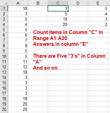
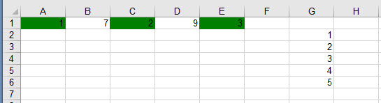
Working with Function =Countif(myRange, Cells(1,1))
In this example "myRange" is a Fixed Range.
-
Sub setcount()
Dim myrange As Range
Dim x As Integer
Dim r As Integer
Dim i As Integer
Set myrange = Application.Range("A1:A20")
r = 1
[E1].Select
For i = 1 To 4
x = Application.WorksheetFunction.CountIf(myrange, Cells(r, 3))
ActiveCell.Value = x
ActiveCell.Offset(1).Select
r = r + 1
Next i
End Sub
Working with Function =Countif(myRange, Cells(1,1))
In this example "myRange" is a Dynamic Range.
-
Sub setcount()
Dim myrange As Range
Dim x As Integer
Dim r As Integer
Dim i As Integer
Dim s As Integer
Dim e As Integer
s = [I2]
e = [J2]
Set myrange = Application.Range(Cells(s, 2), Cells(e, 5))
r = 1
[O1].Select
For i = 1 To 69
x = Application.WorksheetFunction.CountIf(myrange, Cells(r, 14))
ActiveCell.Value = x
ActiveCell.Offset(1).Select
r = r + 1
Next i
End Sub
Add Date and Military Time to Cell
-
Sub Date_and_Time
- Dim ws1 As Worksheet
Set ws1 = Worksheets("Sheet1")
ws1.Range("A1:D1").Merge ' This will merge Cells A1:D1
ws1.Range("A1:A1").Value = "The Date and time is " & Format(Now, "mm/dd/yy hh:Nn") ' Note this is military time.
'You may want to add a "With" statement to size and format the range. Click to see "WITH" Options
Add Date to cell A1 and Time to cell B1 non Military time
-
Sub Date_anTime()
- Dim ws1 As Worksheet
Set ws1 = Worksheets("Sheet1")
ws1.Range("A1:D1").Merge ' This will merge Cells A1:D1
Range("A1").Value = "The Date and time is " & Format(Now, "mm/dd/yy")
Columns("A").AutoFit
Range("b1").Value = Format(Now, "hh:Nn")
Add date and Time 12 hour clock using "With" statement
-
Sub Date_anTime()
-
With Sheet1
.Range("A1").Value = "The Date and time is " & Format(Now, "mm/dd/yy")
.Range("b1").Value = Format(Now, "hh:Nn")
.Columns("A:B").AutoFit
End With
Lastrow
What is in the lastrow.
(Answer 6)
lastRow = Cells(Rows.Count, "A").End(xlUp).Row What is the lastrow (Answer 3)
Lastrow = Application.WorksheetFunction.CountA(Columns(1)) Asking the right question! Makes the difference. |
 |
Find in expanding box
Find Duplicates in a Column of numbers
-
Sub sbFindDuplicatesInColumn()
- Dim lastRow As Long
Dim matchFoundIndex As Long
Dim iCntr As Long
lastRow = Cells(Rows.Count, "D").End(xlUp).Row ' Need to change the Column from "D"
For iCntr = 1 To lastRow
If Cells(iCntr, 4) <> "" Then ' Need to change the Column# where Cells(iCntr,4) is found
matchFoundIndex = WorksheetFunction.Match(Cells(iCntr, 4), Range("D1:D" & lastRow), 0) ' Change the Column#('s) & Letters
If iCntr <> matchFoundIndex Then
Cells(iCntr, 5) = "Duplicate" ' Need to change the Column number to next column to the right
End If
End If
Next
End Sub
Get Data From one workbook and move it to another workbook
-
We will use connections located on the Data tab. Data Tab / Get External Data
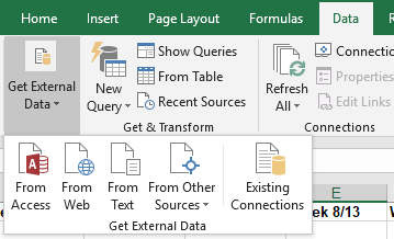
Make a connect to the other excel sheet. If you have too many connection you can delete the ones you do not want from the follow folder(C:\Users\Dan\Documents\My Data Sources)
Copy a Range using PasteSpecial - ( and not using Destination:= )
-
Range("A2:B48").Copy
Range("C2:D48").PasteSpecial Paste:=xlPasteValues, Operation:=xlNone, SkipBlanks _ :=False, Transpose:=False
Copy Data from one workbook, from a dynamic range and paste to another workbook.
-
Sub GetNewData()
Application.ScreenUpdating = False
Dim Target_Workbook As Workbook
Dim Target_Path As String
Dim Master_Workbook As Workbook
Dim Master_Path As String
Dim r As Integer
Dim lastrow As Long
'This is the caregiver file
Target_Path = "E:\Excel\Pam\CaregiverMaxhours.xlsx"
Set Target_Workbook = Workbooks.Open(Target_Path)
r = Cells(Rows.Count, "A").End(xlUp).Row
Range("A2:H" & r).Copy
'This is the Master file
Master_Path = "E:\Excel\Pam\Master.xlsm"
Set Master_Workbook = Workbooks.Open(Master_Path)
lastrow = Cells(Rows.Count, "A").End(xlUp).Row
[a1].Offset(lastrow, 0).PasteSpecial Paste:=xlPasteValues
[a1].Select
Master_Workbook.Save
Target_Workbook.Close
Kill "E:\Excel\Pam\CaregiverMaxhours.xlsx"
Setting the path
-
Sub SaveAsString()
Dim i As Integer
Dim lRow As Integer
Dim sPath As String
Dim sFileName As String
Dim oFilename As String
oFilename = "Book1" ' Change "Book1" to the name of the original book
sPath = ThisWorkbook.Path
lRow = Sheets("Sheet1").Range("A" & Rows.Count).End(xlUp).Row
Application.DisplayAlerts = False
Application.ScreenUpdating = False
For i = 2 To lRow
sFileName = Range("N" & i).Value
ActiveWorkbook.SaveAs Filename:=sPath & "\" & sFileName & ".xlsx", FileFormat:=xlOpenXMLWorkbook, CreateBackup:=False
Next i
Workbooks.Open Filename:=sPath & "\" & oFilename & ".xlsm"
Workbooks.Open Filename:=sPath & "\" & sFileName & ".xlsx"
Application.ScreenUpdating = True
Application.DisplayAlerts = True
ActiveWorkbook.Close
End Sub
Chandoo
Saving a file to the workbook path
-
Dim sPath As String
Dim sFileName As String
sPath = ThisWorkbook.Path ' This is the path of the workbook.
sFileName = Range("N" & i).Value
-
Here is an example, Located at E:\Excel\NotCopyingLastWorkbook
Sub SaveAsString()
Dim i As Integer
Dim lRow As Integer
Dim sPath As String
Dim sFileName As String
sPath = ThisWorkbook.Path
lRow = Sheets("Sheet1").Range("A" & Rows.Count).End(xlUp).Row
Application.DisplayAlerts = False
Application.ScreenUpdating = False
For i = 2 To lRow
sFileName = Range("N" & i).Value
ActiveWorkbook.SaveAs Filename:=sPath & "\" & sFileName & ".xlsx", FileFormat:=xlOpenXMLWorkbook, CreateBackup:=False
Next i
Application.ScreenUpdating = True
Application.DisplayAlerts = True
ActiveWorkbook.Close
End Sub
Select a Range and Selecting and copying a range to a cell
-
Range("A1:C1").Select or .copy
Range("A1", "C1").Select or.copy
Range("A1", Range("C1").End(xlDown)).Copy ' Copies "A1" thru the end of C
Range("A1", Range("A1").End(xlDown)).Copy Range("B1")
Range("A1").CurrentRegion.Copy ' Current Region works but UsedRegion will not.
Copy and paste
- When pasting in VBA use PasteSpecial and then Ctrl+spacebar for additional arguments
Example 1: The word "Destination" does not need to be used
- Worksheets("List").Cells(5, 4).Copy Destination:=Worksheets("Inventory").Cells(r, 14)
Worksheets("List").Cells(5, 4).Copy Worksheets("Inventory").Cells(r, 14) (This should work just as well as the line above it)
Activesheet.Range("A1").Copy Destination:=Range("B1")
Range("A1:A5").copy Destination:=Range("B1")
Dim dt As Object
-
Set dt = Worksheets("List").Cells(2, 8)
dt.Copy
Cells(r, 12).Select ' This selects the cell on the activesheet
Selection.PasteSpecial Paste:=xlPasteValues ' This will paste as a value
Example 2: (Using Special Paste xlPaste Values in a Macro)
-
Dim rng as Range
Dim ws2 as Worksheet
Set rng = Range("A1:D10")
Set ws2 = Worksheets("Sheet2")
rng.Copy
ws2.Cells(Rows.Count, 5).End(xlUp).Offset(1, -2).PasteSpecial xlPasteValues
This will fail.
- rng.Copy Destination:=ws2.Cells(Rows.Count, 5).End(xlUp).Offset(1, -2).PasteSpecial xlPasteValue
This will work: (So we can use Paste Special xlPasteValue)
- rng.Copy
ws2.Cells(Rows.Count, 5).End(xlUp).Offset(1, -2).PasteSpecial xlPasteValues
Copy and paste special (SpecialPaste Values)
- Sub Neworders()
Dim wsI As Worksheet
Dim wsO As Worksheet
Set wsI = Worksheets("Inventory")
Set wsO = Worksheets("Order")
' Application.ScreenUpdating = False
wsO.ListObjects("Table2").DataBodyRange.Copy
wsI.Cells(Rows.Count, 16).End(xlUp).Offset(1).PasteSpecial Paste:=xlPasteValues
wsO.ListObjects("Table2").DataBodyRange.ClearContents
wsO.ListObjects("Table2").Resize Range("A9:D10")
[C10].Formula = "=vlookup([Item '#],Table3,2,0)"
[D10].Formula = "=vlookup([Item '#],Table3,5,0)"
ActiveWorkbook.Save
End Sub
Copy and paste a range column and Transpose to a cell
-
Range("L10:L14").Select
Selection.Copy
Range("M2").Select
Selection.PasteSpecial Paste:=xlPasteAll, Operation:=xlNone, SkipBlanks:= _
False, Transpose:=True
Hide and unHide columns, using a Combobox - Combobox list and target located on Tab "List".
- Here is a Macro to hide and unhide columns based on a ComboBox.
Sub hidcol()
Dim col As Integer
col = [List!B1] + 1
If Worksheets("List").Range("B1") = 27 Then GoTo Line1
Columns(col).EntireColumn.Hidden = True
GoTo Line2
Line1:
Columns("B:AA").EntireColumn.Hidden = True
Line2:
Worksheets("Home").Shapes("Drop Down 5").OLEFormat.Object.Value = 28
End Sub
Sub unhidcol()
Dim col As Integer
col = [List!b2] + 1
If Worksheets("List").Range("B2") = 27 Then GoTo Line1
Columns(col).EntireColumn.Hidden = False
GoTo Line2
Line1:
Columns("B:AA").EntireColumn.Hidden = False
Line2:
Worksheets("Home").Shapes("Drop Down 6").OLEFormat.Object.Value = 28
End Sub
Copy the worksheet into new workbook and Save in a specific folder.
-
Sub sb_Copy_Save_Worksheet_As_Workbook()
Dim wb As Workbook
Set wb = Workbooks.Add
ThisWorkbook.Sheets("Sheet1").Copy Before:=wb.Sheets(1)
wb.SaveAs "C:\temp\test1.xlsx"
End Sub
VBA Course Instruction in PDF
VBA Course home page
How to Password Protect your macro's
- To protect your code, open the Excel Workbook and go to Tools>Macro>Visual Basic Editor (Alt+F11).
Goto: Tools>VBAProject Properties and click "Protection" Check "Lock Project for viewing" and then enter your password and again to confirm it. Click :OK:
http://www.ozgrid.com/VBA/protect-vba-code.htm
How to protect and unprotect a pw protected worksheet or workbook (Tab Review protect sheet/Protect workbook)
- Activesheet.Unprotect "Password"
Activesheet.Protect "Password"
Activeworkbook.Unprotect "Password"
Activeworkbook.Protect "Password"
How to Password Protect / Hide a worksheet and open it using a Macro .
This will allow you to open a workbook which only contains a worksheet named "Menu". The macro on this Menu page will open hidden worksheets using a password.Finally step. Password protect your VBA code as outlined in (How to Password Protect your macro's.) so that no one can open your vba editor and view the macro and its passwords. |
 |
Insert a Row
- Sub inserrt()
'
' inserrt Macro
Rows("3:3").Select
Selection.Insert Shift:=xlDown
End Sub
or
Rows("3:5").EntireRow.Insert
File picker
-
Sub GetFilePathBasic()
' (1) Shows the msoFileDialogFilePicker dialog box.
' (2) Checks if the user picked a file.
' (3) Stores the path to the selected file in a string type variable.
Dim strFilePath As String
With Application.FileDialog(msoFileDialogFilePicker)
' show the file picker dialog box
If .Show <> 0 Then
strFilePath = .SelectedItems(1)
' *********************
' put your code in here
' *********************
' Example: print the path of the selected file to the immediate window
Debug.Print strFilePath ' remove in production
End If
End With
End Sub
Column Name to Column Number
-
Use this macro to find the Column Number Like (A is 1) and (Z is 26) so what is JK? Use the macro to find out.
' To create a keyboard shortcut to this macro click on Developer/Macro/Options
Sub Name2Number()
Dim N As String
N = InputBox("Choose Column Name")
Dim ColName As String
ColName = N
MsgBox Range(ColName & 1).Column, 32, "The Column Number is!..."
End Sub
Using TARGET
- Note Target is used from the "Sheet" module and not the Module
| Private Sub Worksheet_Change(ByVal Target As Range) Application.ScreenUpdating = False If Target.Row > 599 And Target.Column = 2 Then Target.Offset(0, -1) = Date End If Application.ScreenUpdating = True End Sub |
 |
Count number of Rows and Columns
-
Dim lastrow As Integer
Dim lastcol As Integer
lastrow = Cells(Rows.Count, "A").End(xlUp).Row ' Last Row in Column "A"
lastcol = ws1.Cells(1, Columns.Count).End(xlToLeft).Column ' Last Column in Row 1
Dim lColumn As Long
lColumn = ws1.UsedRange.Columns.Count ' Last used Column on worksheet (ws1)
Dim lRow As Long
lRow = ws1.UsedRange.Rows.Count ' Last used Row on worksheet (ws1)
Count the number of non blank cells in a column. Or how many items values or text are in column 2
- Dim lRow As Double
lRow = Application.WorksheetFunction.CountA(Columns(2))
Create a Temp worksheet
- On Error GoTo Line1
Application.DisplayAlerts = False
ThisWorkbook.Sheets("Temp").Delete
Line1:
Application.DisplayAlerts = True
ThisWorkbook.Sheets.Add(After:= _
ThisWorkbook.Sheets(ThisWorkbook.Sheets.Count)) _
.Name = "Temp"
Selecting a column with was chosen with Inputbox
- Dim ltr As String
ltr = InputBox("What column is your data in?", "Date Information")
Dim rng As Range
Set rng = Range(Range(ltr & 1), Range(ltr & 10))
Delete and or Clear Contents in a Row or Column
-
Sub Clear_A_RowsContent()
- Rows("1:1").ClearContents
Sub Clear_A_ColumnsContent()
- Columns("C:C").ClearContents
Sub Clear_A_ColumnsContentUsingInputbox()
Dim x As String
- x = InputBox("Which Row would you like to clear?")
Columns(x).ClearContents
Sub Clear_A_RowsContentUsingInputbox()
- Dim x As Long
x = InputBox("Which Row would you like to clear?")
Rows(x).ClearContents
Sub Delete_A_Row()
- Rows(1).EntireRow.Delete ' This will also Shift Up
Sub Delete_A_Column()
- Columns("A").Delete ' This will also Shift:=xlLeft
Sub Delete_A_ColumnUsingInputbox()
- Dim x As String
x = InputBox("Which Column would you like to delete?")
If IsNumeric(x) Then GoTo Line1
Columns(x).Delete
GoTo Line2
- MsgBox "Please enter Text only"
End Sub
Sub Delete_A_RowUsingInputbox()
- On Error GoTo Line1
Dim x As Long
x = InputBox("Which Row would you like to delete?")
Rows(x).EntireRow.Delete ' This will also Shift:=xlUp
GoTo Line2
- MsgBox "Please enter Numbers only"
End Sub
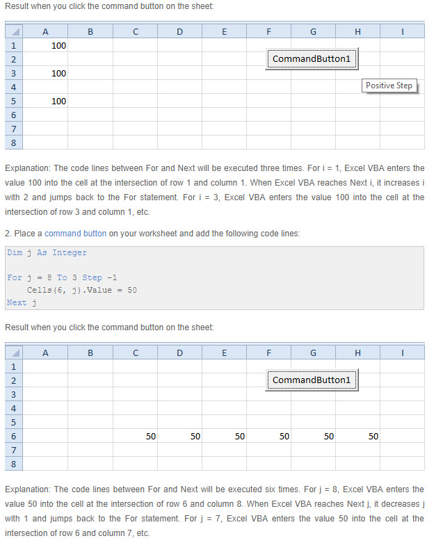
Loop, skipping cells. (More on Loops)
- Dim i As Integer
For i = 1 To 6 Step 2
Cells(i, 1).Value = 100
Next i
Case / Example
- Sub pik()
Dim intValue As Integer
intValue = InputBox("Enter value")
Select Case intValue
Case 1
MsgBox "Aircraft"
Case 2
MsgBox "AutoMobile"
Case 3
MsgBox "SnowMobile"
Case Else
Debug.Assert False
End Select
End Sub
Last Row in Column "A"
-
Dim r As Long
r = Cells(Rows.Count, "A").End(xlUp).Row
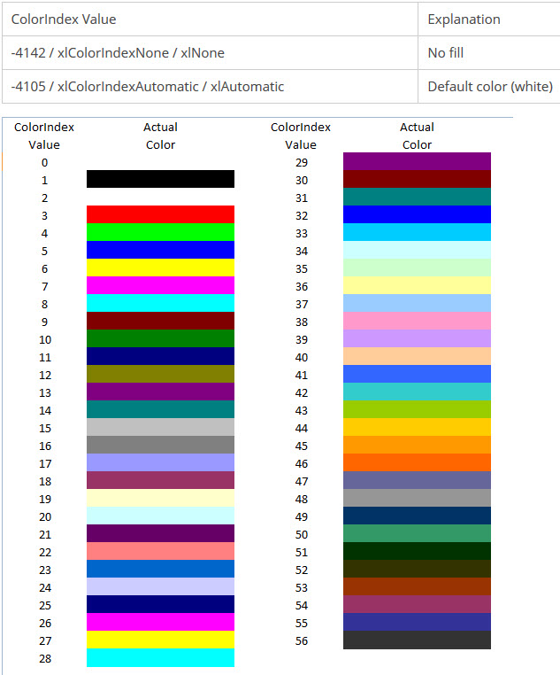
Link to Microsoft Color Index
Change font color to red of all numbers in column "A" based on input number.
-
Sub colr()
- Dim i As Long
Dim r As Long
Dim x As Long
x = InputBox("Enter number", "Red number below")
Columns(1).Font.Color = vbBlack
r = Cells(Rows.Count, "A").End(xlUp).Row
For i = 1 To r
- If Cells(i, 1).Value < x Then
Cells(i, 1).Font.Color = vbRed
End If
If Interior ColorIndex is then? - Hex to RGB converter
-
Sub CellColors()
'
' So you may want to use these examples instead of using conditional formatting because
'you can not determine the interior color of a conditionally formatted cell
Range("A1").Interior.ColorIndex = 11 ' This will change the interior color TO 11 = Dark Blue
Range("A1").Font.ColorIndex = 3 ' This will change the FONT color to 3 is red
Range("A1").Interior.ColorIndex = -4142 ' This will reset the cell interior to NO FILL
Range("A1").Interior.ColorIndex = -4105 ' This will reset the cell interior to White
' What the difference between -4142 and -4105
'-4105 fills the interior White so in you will not see the Guideline between "A1" and "B1" where as -4142 resets to no fill like a new sheet looks.
Range("A1").ClearContents ' This will clear the content of the cell
Range("A1").ClearFormats ' This will clear the Formatting of the cell
If Range("A1").Interior.ColorIndex = 56 Then ActiveCell.Offset(0, 1).Select ' 56 = Dark Green
If Range("A1").Interior.ColorIndex = 56 Then Range("A2:H2").Interior.ColorIndex = 3 ' 3 = Red - This changes the color of a range of cells.
End Sub
What color is the ActiveCell ?
- Sub test_color()
MsgBox ActiveCell.Interior.ColorIndex
End Sub
Setting the interior color of a cell based on Criteria
-
(----------------This could be use like conditional formating--------------)
Sub ConditionalColorChange()
Dim r As Integer
Dim c As Integer
Dim r1 As Integer
Dim c1 As Integer
Dim i As Integer
r = 1
c = 1
r1 = 2
Range("A1:E1").ClearFormats
Cells(1, 1).Select
For i = 1 To 5
Do Until IsEmpty(ActiveCell)
If Cells(r, c) = Cells(r1, 7) Then
With ActiveCell
.Interior.Color = RGB(0, 128, 0)
Exit Do
End With
End If
ActiveCell.Offset(0, 1).Select
c = c + 1
Loop
Cells(1, 1).Select
c = 1
r1 = r1 + 1
Next i
MsgBox "Finished!"
End Sub
Here we see Cells "A1", "C1" & "E1" changed to Green because those numbers were found in Column "G".
Todays date is (Variable Name (TDay))
-
Sub tdat()
Dim TDay As String
TDay = Date
MsgBox TDay ' This will show Todays Date
End Sub
Add Todays Date to cell A1 then add days to that date in cell below it.
Working with Dates ... Click here for more.
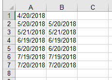 |
Sub addnumbers() Dim startdate As Date Dim newdate As Date Dim r As Integer startdate = Date Range("A1") = startdate r = 30 newdate = DateAdd("d", r, startdate) Range("A2") = newdate r = 31 newdate = DateAdd("d", r, startdate) Range("A3") = newdate r = 60 newdate = DateAdd("d", r, startdate) Range("A4") = newdate r = 61 newdate = DateAdd("d", r, startdate) Range("A5") = newdate r = 90 newdate = DateAdd("d", r, startdate) Range("A6") = newdate r = 91 newdate = DateAdd("d", r, startdate) Range("A7") = newdate End Sub |
Delete Duplicates in a Range
-
Sub Remove_Duplicates()
With ActiveSheet
- .Range("A1:N" & .Cells(Rows.Count, 14).End(xlUp).Row).RemoveDuplicates
End With
End Sub
Download a txt file from the internet and save in file E:\Lotto. (used in Lotto_Fun 7)
-
Sub GetPBallNumbers()
Dim db As Worksheet
Set db = Worksheets("DB")
Kill "E:\Lotto\Winnums-Text.txt"
Dim myURL As String
myURL = "http://www.powerball.com/powerball/winnums-text.txt"
Dim WinHttpReq As Object
Set WinHttpReq = CreateObject("Microsoft.XMLHTTP")
WinHttpReq.Open "GET", myURL, False
WinHttpReq.Send
Dim oStream As Variant
myURL = WinHttpReq.ResponseBody
If WinHttpReq.Status = 200 Then
Set oStream = CreateObject("ADODB.Stream")
oStream.Open
oStream.Type = 1
oStream.Write WinHttpReq.ResponseBody
oStream.SaveToFile ("E:\Lotto\Winnums-Text.txt")
oStream.Close
End If
Dim rng As Range
Set rng = Range("A:A")
Dim col As Long
col = Application.WorksheetFunction.CountA(rng)
db.Range("K3:Q" & col).ClearContents
db.Range("A:I").ClearContents
Call ImportDataTxT
[A1].End(xlDown).Offset(0, 9).Select
Dim i As Integer
For i = 1 To 7
ActiveCell.Offset(0, 1).Select
Range(Selection, Selection.End(xlUp)).FillDown
Next i
End Sub
Create a new Worksheet using VBA
-
Sub CreateSheet()
Dim nwsht As Variant
nwsht = InputBox("Enter name of new Sheet")
With ThisWorkbook
.Sheets.Add(After:=.Sheets(.Sheets.Count)).name = nwsht
End With
End Sub
Create new Worksheets for all names listed in column "A" on Sheet("Sched")
-
Sub AddSheet()
With Worksheets("Sched")
Dim lastrow As Long
lastrow = .Cells(.Rows.Count, "A").End(xlUp).Row
Dim i As Long
For i = 1 To lastrow
If IsError(Application.Evaluate("'" & .Cells(i, 1).Value & "'!A1")) And .Cells(i, 1) <> "" Then
Dim ws As Worksheet
Set ws = ThisWorkbook.Worksheets.Add
ws.name = .Cells(i, 1).Value
End If
Next i
End With
End Sub
Control a table filter with a macro.
-
Here is the setup by Tabs:
- Home Tab, will display results.
DB Tab, will contain the data base information. AKA Table 1
List Tab, will duplicate the DB informaton. In this case Table 4
List2 Tab will house the Combo box data and logic. Table 6
The macro:
-
Sub startmigration()
Dim wsD As Worksheet
Dim wsL As Worksheet
Dim wsH As Worksheet
Dim wsL2 As Worksheet
Dim x As Long
Set wsD = Worksheets("DB")
Set wsL = Worksheets("List")
Set wsH = Worksheets("Home")
Set wsL2 = Worksheets("List2")
x = wsL2.[D1]
wsH.Range("B2:J100").Delete
wsL.ListObjects("Table4").DataBodyRange.ClearContents
wsD.ListObjects("Table1").DataBodyRange.Copy Destination:=wsL.Range("A2")
wsD.Range("Table1[Invoice '#]").Copy Destination:=wsL2.Range("A2")
wsL2.Range("A1").CurrentRegion.RemoveDuplicates Columns:=1
wsL.ListObjects("Table4").Range.AutoFilter Field:=1, Criteria1:=x
wsL.ListObjects("Table4").DataBodyRange.Copy Destination:=wsH.Range("B2")
wsH.Columns("B:L").AutoFit
End Sub
(This macro also needs the following macro to refresh the invoice list when something is added to the database)
Here is a newer example of controlling the filter
-
Sub lookup() 'This macro gets the data from table 1
Dim r As Double
Dim x As Double ' if you get an error change Double to String
Dim wsL As Worksheet
Dim wsD As Worksheet
Dim wsH As Worksheet
Set wsL = Worksheets("List")
Set wsD = Worksheets("DB")
Set wsH = Worksheets("Home")
r = wsL.[C1]
x = wsL.Cells(r, 1)
Application.ScreenUpdating = False
wsH.Range("B2:J50").Delete
wsD.ListObjects("Table1").Range.AutoFilter Field:=1, Criteria1:=x
wsD.ListObjects("Table1").DataBodyRange.Copy Destination:=wsH.Range("B2")
wsH.Columns("B:J").AutoFit
End Sub
Sub GetInvoiceNumbers() ' This macro gets the invoice numbers from table 1 then remove the duplicates so that we can use the number in a combo-box
Dim wsD As Worksheet
Dim wsL As Worksheet
Set wsD = Worksheets("DB")
Set wsL = Worksheets("List")
Application.ScreenUpdating = False
wsD.ListObjects("Table1").ListColumns(1).Range.Copy Destination:=wsL.Cells(1, 1)
wsL.Range("A1").CurrentRegion.RemoveDuplicates Columns:=1
End Sub
Sub resetDB() 'This macro resets the main data in table 1 on sheet "DB"
Dim wsD As Worksheet
Set wsD = Worksheets("DB")
wsD.ListObjects("Table1").Range.AutoFilter Field:=1
End Sub
This was used in Excel File: " Autofilter_ControlledByVBA"
Slicer ... This will Clearing the slicer filter.
-
Sub ClearSlicer()
-
ActiveWorkbook.SlicerCaches("Slicer_Name").ClearManualFilter
ActiveWorkbook.SlicerCaches("Slicer_CareGiver").ClearManualFilter
ActiveWorkbook.SlicerCaches("Slicer_Weeks").ClearManualFilter
ActiveWorkbook.SlicerCaches("Slicer_Month").ClearManualFilter
ActiveWorkbook.SlicerCaches("Slicer_Year").ClearManualFilter
Clearing a Table Filters
-
Sub TableFilterClear()
'
' TableFilterClear Macro
'
ActiveSheet.ListObjects("Table2").Range.AutoFilter Field:=1
ActiveSheet.ListObjects("Table2").Range.AutoFilter Field:=2
ActiveSheet.ListObjects("Table2").Range.AutoFilter Field:=3
ActiveSheet.ListObjects("Table2").Range.AutoFilter Field:=4
End Sub
Table Filter ... Setting a specific filter in a Field/Column
-
ActiveSheet.ListObjects("Table3").Range.AutoFilter Field:=1, Criteria1:= _
"David Duncan" 'Specifies David Duncan in field/column 1
ActiveSheet.ListObjects("Table3").Range.AutoFilter Field:=2, Criteria1:= _
"39" 'Specifies 39 in field/Column 2
AutoFilter with 2 criteria
- Here we are concatenating "<" & date1 and ">" & date2 (in blue text below)
Sub picr()
Dim r As Integer
Dim wsml As Worksheet
Dim wspp As Worksheet
Dim date1 As Date
Dim date2 As Date
Set wsml = Worksheets("Member_List")
Set wspp = Worksheets("PayPeriods")
r = wsml.[A1]
date1 = wspp.Cells(r, 1)
date2 = wspp.Cells(r, 2)
Application.ScreenUpdating = False
wsml.ListObjects("Table1").Range.AutoFilter Field:=3, Criteria1:= _
">" & date1, Operator:=xlAnd, Criteria2:="<" & date2
[A1].Select
End Sub
Reset AutoFilter on Table 1 in Field 3
-
Sub ResetAutoFilter()
- ActiveSheet.ListObjects("Table1").Range.AutoFilter Field:=3
End Sub
Select Current Region and remove duplicates
- Sub Updatedatabase()
Dim wsL2 As Worksheet
Dim wsD As Worksheet
Set wsL2 = Worksheets("List2")
Set wsD = Worksheets("DB")
wsD.Range("Table1[Invoice '#]").Copy Destination:=wsL2.Range("A2")
wsL2.Range("A1").CurrentRegion.RemoveDuplicates Columns:=1
End Sub
You will use this macro when you add a new item to the database Tab DB. Download the speadsheet here this was based on here.
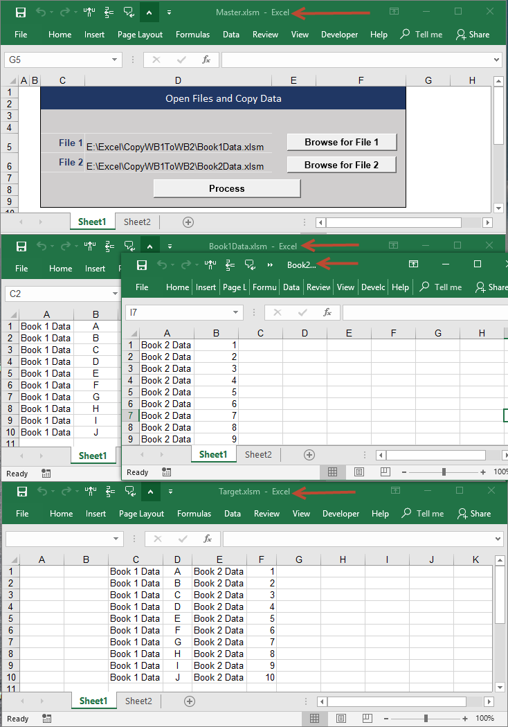
How to copy and paste from one workbook to another workbook
-
How this works. There will be a Master Workbook that will allow you to choose up to two other workbooks in a directory and move data from those workbooks to a Target workbook which has a know location.
Code for all 3 macros: (Look up a file location on the computer)
-
Sub sbVBA_To_Choose_Workbook1()
Dim strFileToOpen As String
strFileToOpen = Application.GetOpenFilename _
(Title:="Please choose a file to open", _
FileFilter:="Excel Files *.xlsm* (*.xlsm*),")
If strFileToOpen = "False" Then
MsgBox "No file selected.", vbExclamation, "Sorry!"
Exit Sub
Else
Range("D5") = strFileToOpen
End If
End Sub
Sub sbVBA_To_Choose_Workbook2()
Dim strFileToOpen As String
strFileToOpen = Application.GetOpenFilename _
(Title:="Please choose a file to open", _
FileFilter:="Excel Files *.xlsm* (*.xlsm*),")
If strFileToOpen = "False" Then
MsgBox "No file selected.", vbExclamation, "Sorry!"
Exit Sub
Else
Range("D6") = strFileToOpen
End If
End Sub
Sub sbMainProcess() ' thiswill open the filed that you just looked up.
Dim wbSource1, wbSource2, wbTarget
If Cells(5, 4) = "" Then GoTo Line1 ' If no file name is in File 1 then exit
If Cells(6, 4) = "" Then GoTo Line2 ' If no file name is in File 2 only process File 1
'Open 1 files
Set wbSource1 = Workbooks.Open(Range("D5"))
ThisWorkbook.Activate
Set wbSource2 = Workbooks.Open(Range("D6"))
ThisWorkbook.Activate
Set wbTarget = Workbooks.Open("E:\Excel\CopyWB1ToWB2\Target") 'Change this
'Now Copy the Data
' ----Note!----- You will need to change the Range locations and Destination Ranges
wbSource1.Sheets("Sheet1").Range("A1:B10").Copy Destination:=wbTarget.Sheets("Sheet1").Range("C1")
wbSource2.Sheets("Sheet1").Range("A1:B10").Copy Destination:=wbTarget.Sheets("Sheet1").Range("E1")
'Now Close the Files
wbSource1.Close
wbSource2.Close
GoTo Line3
Line2:
'Open 1 files
Set wbSource1 = Workbooks.Open(Range("D5"))
ThisWorkbook.Activate
Set wbTarget = Workbooks.Open("E:\Excel\CopyWB1ToWB2\Target") 'Change this
'Now Copy the Data
wbSource1.Sheets("Sheet1").Range("A1:B10").Copy Destination:=wbTarget.Sheets("Sheet1").Range("C1")
'Now Close the Files
wbSource1.Close
GoTo Line3
Line1:
MsgBox "No File was choosen. Please choose a file."
Line3:
'Save the Target File
wbTarget.Save
'Save the Target File
wbTarget.Close
End Sub
Open a Excel workbook (file) from an existing workbook
-
Sub sbVBA_To_Choose_Workbook1()
Dim wbSource1
Dim strFileToOpen As String
strFileToOpen = Application.GetOpenFilename _
(Title:="Please choose a file to open", _
FileFilter:="Excel Files *.xlsm* (*.xlsm*),")
If strFileToOpen = "False" Then
MsgBox "No file selected.", vbExclamation, "Sorry!"
Exit Sub
Else
Set wbSource1 = Workbooks.Open(strFileToOpen)
End If
End Sub
How to: Create / Delete a folder or delete a file in a folder
- Sub Make_Dir_on_G()
MkDir "G:\DannyBoy" ' This will create a folder named DannyBoy on Drive G:\
End Sub
Sub Remove_Dir_on_G()
RmDir "G:\DannyBoy" ' This will remove the folder DannyBoy on drive G:\
End Sub
Sub Delete_all_txt_files()
Kill "G:\DannyBoy\*.txt" ' This will delete all .txt files found in G:\DannyBoy folder
End Sub
How to create a folder with a inputbox and then copy a file using the FileCopy from one folder to another using the Inputbox
- Original folder is Dano.
#1 Will create a folder in Dano using the inputbox to name for folder. If the folder name already exist, you will get a messagebox error.
#2 Will copy a pre existing file named templa.xlsm to a folder specified by the inputbox.
-
#1
Sub filefolder()
- Dim name As String
name = InputBox("Create new file in C:\Dano")
If Len(Dir("c:\Dano\" & name, vbDirectory)) = 0 Then
MkDir "c:\Dano\" & name
Exit Sub
End If
MsgBox "Sorry that name already exists please try again"
End Sub
#2
Sub copytemplate()
'
- Dim frompath As String
Dim topath As String
Dim name As String
name = InputBox("Name to put template in?")
frompath = "C:\Dano\Templa.xlsm"
topath = "C:\Dano\" & name & "\" & name & ".xlsm"
FileCopy frompath, topath
End Sub
Using CountA
- Application.WorksheetFunction.CountA(A:A) (or A:A can be a variable)
Dim rng as range
Dim r as long
set rng = Range("A:A")
r = Application.WorksheetFunction.CountA(rng)
Count even and odd numbers in a range using the MOD operator
-
MOD is the remainder of two number. Thus
- 14 MOD 4 = 2
8 MOD 5 = 3
14 divide by 4 or (4 * 3 =12) with a remainder of 2
8 divide by 5 or (5 * 1 = 5) with a remainder of 3
20 Mod 2 = 0
21 Mod 2 = 1
If the value 20 is MODed by 2 then the result would be 0. Since 2 divides into 20 evenly. we know that we have an even number. IF there is a remainder of anything else than zero we are dealing with an Odd number.
To check if a value is an even or an odd number I used the Mod operator to divide the variable by 2. If the result returned 0 then it must be an even number. And if not then it must be an odd number.
Find if cell "A1" is even or odd. Note a Blank cell is considered "Even"
Sub oddevn()
If Cells(1, 1) Mod 2 = "0" Then
MsgBox "Cells is Even"
Else
MsgBox "Cells is odd"
End If
End Sub
Functions (application.WorksheetFunction. ?)
Functions - VBA w/Sub Example:
-
Function Celsius(dan)
Celsius = (dan - 32) * 5 / 9
End Function
Sub tempconversion()
Dim temp As Variant temp = Application.InputBox(Prompt:= _ "Please enter the temperature in degrees F.", Type:=1) MsgBox "The temperature is " & Celsius(temp) & " degrees C."
End Sub
Note! the word "dan" was originaly "fDegrees". Deleting "dan" or "fDegrees" and the macro will fail.
More example of Functions.
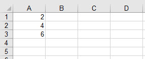
- Function Area(x As Long, y As Long) ' Note that in the parentheses could be a Range, This is like Dim in a Sub - Like Dim x As Long
Area = x - y ' Note this could be + , - , / , * This is the actual function which can be called with the key word "Area"
End Function
Sub nex() ' Find more on Functions at: http://www.excel-easy.com/vba/function-sub.html
Dim z As Long
z = Area([A1], [B1])
[D1].Value = z
'MsgBox z
End Sub
This places the answer to the equation in cell D1.
| A | B | C | D | |
| 1 | 10 | 6 | 4 | |
| 2 | ||||
| 3 |
Types of Variables
| Name | Type | Details | Symbol |
| Byte | Numerical | Whole number between 0 and 255. | |
| Integer | Numerical | Whole number between -32'768 and 32'767. | % |
| Long | Numerical | Whole number between - 2'147'483'648 and 2'147'483'647. | & |
| Currency | Numerical | Fixed decimal number between -922'337'203'685'477.5808 and 922'337'203'685'477.5807. | @ |
| Single | Numerical | Floating decimal number between -3.402823E38 and 3.402823E38. | ! |
| Double | Numerical | Floating decimal number between -1.79769313486232D308 and 1.79769313486232D308. | # |
| String | Text | Text. | $ |
| Date | Date | Date and time. | |
| Boolean | Boolean | True or False. | |
| Object | Object | Microsoft Object. | |
| Variant | Any type | Any kind of data (default type if the variable is not declared). |
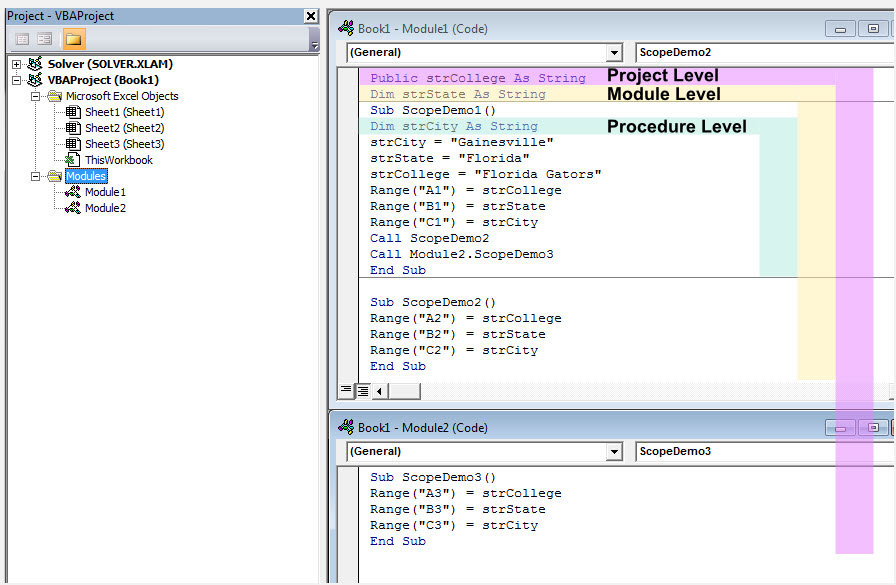
Scope of Variable
 |
Hiding Rows
- Rows.EntireRow.Hidden = True or False to unhide
| Example: Sub hidrow() Dim BeginRow As Integer Dim EndRow As Integer Dim ChkCol As Integer Dim RowCnt As Integer Dim r As Integer Dim box As Integer BeginRow = 10 EndRow = 205 ChkCol = 2 r = 1 Application.ScreenUpdating = False For box = 1 To 5 ' this represents the number of check boxes being used For RowCnt = BeginRow To EndRow If Cells(r, 1) = True Then If Cells(BeginRow, ChkCol).Value = Cells(r, 2) Then Cells(BeginRow, ChkCol).Rows.EntireRow.Hidden = True End If End If If Cells(r, 1) = False Then If Cells(BeginRow, ChkCol).Value = Cells(r, 2) Then Cells(BeginRow, ChkCol).Rows.EntireRow.Hidden = False End If End If BeginRow = BeginRow + 1 Next RowCnt r = r + 1 BeginRow = 10 EndRow = 30 Next box End Sub |
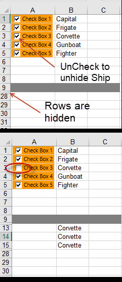 |
If statement that stops or ends the macro operation.
- If [a1] > "6" Then Exit Sub
Moving Up, Down, Left, Right
-
.end.(xlup)
.end.(xlDown)
.end.(xlToRight)
.end.(xlToLeft)
Selection.End(xlDown).select
Activecell.offset(Row, Column).select
Find next blank cell in Column "B"
- Cells(ActiveSheet.Rows.Count, 2).End(xlUP).Offset(1 ,0).Select
Fill in the "Blanks" or other value in a Contiguous range that contains blank cells
-
Range("A1").CurrentRegion.SpecialCells(xlCellTypeBlanks).Value = "Blank"
| A | B | C | D | |
| 1 | Dan | Edie | Blank | Blank |
| 2 | Blank | Amanda | Bella | Blank |
| 3 | Blank | Blank | Blank | Patrick |
| 4 | ||||
| 5 |
Fill blanks with cell above
| Start with: |
Finish with: |
Select a Range and Selecting and copying a range to a cell
-
Range("A1:C1").Select or .copy
Range("A1", "C1").Select or.copy
Range("A1", Range("C1").End(xlDown)).Copy ' Copies "A1" thru the end of C
Range("A1", Range("A1").End(xlDown)).Copy Range("B1")
Range("A1").CurrentRegion.Copy ' Current Region works but UsedRegion will not.
Select a "CurrentRegion"
- Current Region = A contiguous range of cells. Total and 100 will not be selected.
-
Range("A1").CurrentRegion.SpecialCells(xlCellTypeBlanks).Value = "Blank"
| A | B | C | D | |
| 1 | Dan | Edie | ||
| 2 | Amanda | Bella | ||
| 3 | Patrick | |||
| 4 | ||||
| 5 | Total | 100 |
Select a "Used Range"
- Used Range. All data is select regardless of the blank cells in Row 4. This is only used on a Sheets not from a cell range.
- Sheet1.UsedRange.Select
| A | B | C | D | |
| 1 | Dan | Edie | ||
| 2 | Amanda | Bella | ||
| 3 | Patrick | |||
| 4 | ||||
| 5 | Total | 100 |
Select Used Range and activate cell "B5"
- Sheet1.UsedRange.Cells(Sheet1.UsedRange.Rows.Count, 1).Offset(1, 0).Select
| A | B | C | D | |
| 1 | ||||
| 2 | Dan | Edie | ||
| 3 | Amanda | Patrick | ||
| 4 | Bella | |||
| 5 |
Using "With" to choose a cell and set a value in a cell
-
Sub UsingWith ( )
With Worksheets(2).Range("C5") 'Chooses cell "C5"
- .Value = "Enter Number" ' Puts text "Enter Number" in cell "C5"
.Offset(1).Value = "1" 'Offsets from "C5" one cell down to "C6" and enter number "1"
.Offset(1).Resize(10).DataSeries Step:=1 'Offsets from "C6" and repeats 10 times one "Step" at a time
.Cells(ActiveSheet.UsedRange.Rows.Count, 1).Offset(1, 0).Select 'Activecell is moved to location "C16"
End Sub
'So it's like adding each of the dot lines to the original statement. Also note that we only used "Select" one time. This helps with keeping the macro fast.
Using "With" to format a range of cells
Sub FontBorderColor()
.Font.Name = "Arial" .Font.Bold = True .HorizontalAlignment = xlCenter (Left or Right) .VerticalAlignment = xlBottom (Center or Top) .Font.Color = RGB(255, 255, 255) .Font.Size = 18 .Font.Italic = True .Font.Underline = True .Borders.Weight = 2 ' Use this to set cell borders .Borders.Color = RGB(217, 255, 196) .Interior.Color = RGB(68, 114, 196) End With End Sub |
Sub colorOutSideBorderFont2() With Range("A3:E3") .Font.Bold = True .Font.Color = RGB(255, 21, 0) ' RGB = Red .BorderAround ColorIndex:=3, Weight:=xlThin ' or xlThick End With End Sub |
Fill Down
- Range(ActiveCell, ActiveCell.End(xlUp)).FillDown
Range(Selection, Selection.End(xlUp)).Select
Selection.filldown
Fill Down Example
-
(In Cell "A1" put number "1" In Cell "B1" put number "2")
Sub fil()
Dim SourceRange As Range
Dim fillRange As Range
Set SourceRange = Worksheets("Sheet1").Range("A1:A2")
Set fillRange = Worksheets("Sheet1").Range("A1:A22")
SourceRange.AutoFill Destination:=fillRange
End Sub
Flash fill (Fill down)
-
Range("$A$1").flashfill
' This will fill down to adjacent column. Set up Column "B" enter 1 thru 10. Cell "A1" enter "1". Run macro.
Setting Row Height and Column Width
- Sub wide()
- Columns("A:E").ColumnWidth = 25
Rows("1:10").RowHeight = 25
Goto last Row in a specified Column
-
FinalRow = Cells(Rows.Count, 2).End(xlUp).Select '
This will take you to the last cell in column 2.
FinalRow = Cells(Rows.Count, 2).End(xlUp).Offset(1).Select ' This will take you to the last cell in column 2 and offset to the next open cell down.
Goto last Row in column "A" using a (Control box using Sheet2 Cell B1 (Dan))
- Sub lstrow()
Dim x As Integer
x = Worksheets("Sheet2").Range("B1") + 3
FinalRow = Cells(Rows.Count, x).End(xlUp).Offset(1).Select
End Sub
| A | B | C | D | |
| 1 | Dan | Edith | ||
| 2 | Amanda | |||
| 3 | ||||
| 4 | ||||
| 5 |
Goto last Column "C" cell using a (Control box using Sheet2 Cell B1(Dan))
-
Sub LCol()
Dim x As Integer
x = Worksheets("Sheet2").Range("B1")
FinalColumn = Cells(x, Columns.Count).End(xlToLeft).Offset(0, 1).Select
End Sub
| A | B | C | D | |
| 1 | Dan | Edith | ||
| 2 | Amanda | |||
| 3 | ||||
| 4 | ||||
| 5 |
Goto the end of a Row using a drop down list of names regardless of order.
- Sub go2DBcol()
- Dim r As Long
Dim wsH As Worksheet
Dim wsD As Worksheet
Dim wsL As Worksheet
Set wsH = Worksheets("Home")
Set wsD = Worksheets("DB")
Set wsL = Worksheets("List")
r = Application.WorksheetFunction _
.Match(wsH.Range("B3"), wsD.Range("A:A"), 0)
With wsD
.Cells(r, Columns.Count).End(xlToLeft).Offset(0, 1).Value = "NewCell"
End With
End Sub
another example (x = WorksheetFunction.Match(0, Range(Cells(1, 1), Cells(10, 1)), 0))
DropDown list is located on Tab "Home" "Cell B3".
This can also paste a range to the end of the row.
- Sub go2DBcol()
Dim r As Long
Dim wsH As Worksheet
Dim wsD As Worksheet
Dim wsL As Worksheet
Dim x As Range
Set wsH = Worksheets("Home")
Set wsD = Worksheets("DB")
Set wsL = Worksheets("List")
r = Application.WorksheetFunction _ .Match(wsH.Range("B3"), wsD.Range("A:A"), 0)
Set x = wsH.Range("A1").CurrentRegion
x.Copy
With wsD
.Cells(r, Columns.Count).End(xlToLeft).Offset(0, 1).PasteSpecial Paste:=xlPasteValues
End With
x.ClearContents
End Sub
Open a word docx from excel
-
Sub opnworddoc()
Dim objWord As Object
Set objWord = CreateObject("Word.Application")
objWord.Visible = True
'Change the directory path and file name to the location
'of the document you want to open from Excel
objWord.Documents.Open "E:\Excel\StackOverFlow\WorkProfile.docx"
End Sub
Selecting cells with "Resize" and then taking action on them.
- Sub resize()
- 'Range("A1").resize(Row,Column).Select or ClearContents or what ever.
'Range("A1").resize(Rowsize:=4, ColumnSize:=4).Select 'Select from A1 4 row and 4 columns
'Range("A1").resize(2).Select ' Selects from A1 2 row or Cells A1 and A2
Range("A1").resize(2,0).ClearContents ' This clears the contents of Cells A1 and A2
| A | B | C | D | |
| 1 | Dan | |||
| 2 | Edith | |||
| 3 | ||||
| 4 | ||||
| 5 |
Convert a range of formula's to Values
- Sub ChangeToValue()
- Dim rngcol As Range
Set rngcol = Range("D:D") 'Set the range to Column "D"
rngcol.Value = rngcol.Value 'Change the copied formula('s) from "C" to column "D" to values.
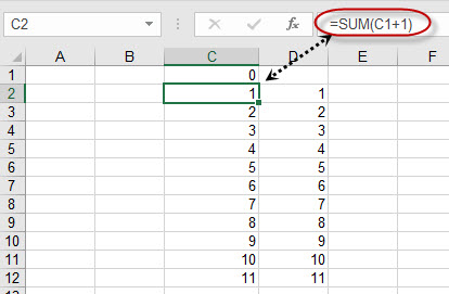 |
Cells in column "C" are formulas. Once we copy the formula to Column "D" we can now use the macro to convert the formula's in column "D" to values. |
On Error handling. (Read more about error handling)
-
On Error GoTo ErrorHandler
ErrorHandler:
On Error GoTo Line1 ' you can change 1 to any number.
Line1:
On Error Resume Next ' This will skip the error and continue on with the next line of code in the macro.
Example:
- Sub fillblanks()
On Error Resume Next
Range("A1").CurrentRegion.SpecialCells(xlCellTypeBlanks).Value = 0 ' there are no blank cells to fill so the error is skipped
'The macro continues from here.
End Sub
Skipping lines inside a macro
- Sub go2()
- If Range("A1") = 1 Then
GoTo Line1
Else
GoTo Line2
End if
Line1:
MsgBox "This is line 1"
GoTo Line3
Line2:
MsgBox "Range A1 does is not number 1"
Exit Sub
Line3:
MsgBox "You just skipped Line2. This macro will now end"
End Sub
Using Case
- Sub Using_case()
- Dim score As Integer
Dim result As String
score = InputBox("Enter Score")
Range("A1").Value = score
Select Case score
Case Is >= 80
result = "very good"
Case Is >= 70
result = "good"
Case Is >= 60
result = "sufficient"
Case Else
result = "poor"
End Select
Range("B1").Value = result
End Sub
Test for Duplicates
- Sub TestForDuplicates()
'PURPOSE: Determine if duplicate values exist in a provided range
'SOURCE: www.TheSpreadsheetGuru.com/the-code-vault
Dim rng As Range
Dim myArray As Variant
'Store Range to search through
Set rng = Range("A1:A3")
'Use Unique Function and store result to an Array variable
myArray = WorksheetFunction.Unique(rng)
'Test Range for Duplicates
If UBound(myArray) < rng.Count Then
MsgBox "Duplicates Found! Aborting..."
Else
MsgBox "No Duplicates Found. Continuing on..."
End If
End Sub
Age What is my age
What does ME mean?
-
What is Me?
Me refers to the parent object from which the code is "sitting" in. For a UserForm, when you are writing the code within the UserForm module,
Me will refer to that UserForm. Similarily, if you are writing in a Sheet module, the Me will refer to that specific sheet.
Using Me is handy because we don't have to worry about the sheet name changing, and it also makes it a little easy for future code readers as
they don't have to remember that "Main UserForm" is the UserForm we are currently working on. You can apply the same methods to the Me
that you would be able to apply to the object if you gave the full name.
Note!, that ("Me.") can only be used in a Sheet not in a Module.
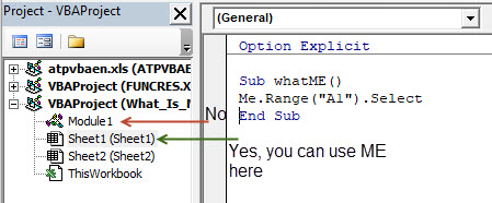
Within the Sheet1 module, the following lines are identical in purpose
Worksheets("Sheet1").Range("A1").Select
Me.Range("A1").Select
Events
-
Private Sub Workbook_open() ' This will trigger when the WorkBook is opened.
- MsgBox "Welcome Back!"
End Sub
Private Sub Worksheet_Change(ByVal Target As Range) ' This will trigger any time a cell has changed
MsgBox "Hello, The macro just triggered"
End Sub
Private Sub Worksheet_Calculate()' This will Trigger on an Calculation event
MsgBox "Just recalulated"
End Sub
More Events at Tutorpoint.com
Searchable Dropdown List using ActiveX combobox
-
See file "ActiveSearchDropdownList.xlsm" in excel.
Instruction on the web at: Click Here. Watch the video.
VBA Wait Application Method: Example 1
- Please find the below example for Wait method of application object in excel VBA.
Application. The below macro Pauses an application till 4.00 PM today.
Sub Appl_Wait1()
Application.Wait "16:00:00"
End Sub
VBA Wait Application Method: Example 2
- Please find the below example for Wait method of application object in excel VBA.
Application. The below macro Pauses an application for 20 seconds from now.
Sub Appl_Wait2()
Application.Wait Now + TimeValue("00:00:20") ' I used this one in lotto xlPlus
End Sub
VBA Wait Application Method: Example 3
-
Please find the below example for Wait method of application object in excel VBA.
‘Display message after 60 seconds.The below macro displays a message like “Your session has expired”
after 60 seconds or 1 hour.
Sub Appl_Wait3()
If Application.Wait(Now + TimeValue("0:00:60")) Then
MsgBox "Your session has expired"
End If
End Sub
VBA Wait Application Method2: Example 4 Less than 1 second
-
Sub TestTimer()
Dim t As Double
t = Timer
Do Until Timer - t >= 0.25
Loop
End Sub